Lake Malawi cichlid pangenome graph reveals extensive structural variation driven by transposable elements

Long-read assemblies and graph construction

SNP studies have provided support for the categorization of Lake Malawi cichlids into seven ecomorphological groups (Fig. 1A; Malinsky et al. 2018): (1) the littoral, rock dwelling “mbuna”; (2) the river and swamp-dwelling Astatotilapia calliptera; (3) benthics in shallow areas; (4) benthics in deep areas; (5) the “utaka”; and the pelagic groups (6) Diplotaxodon and (7) Rhamphochromis. For this study, six long-read assemblies were newly prepared for five species, specifically one mbuna (Tropheops sp. “mauve”), three benthic (Aulonocara stuartgranti, Otopharynx argyrosoma, Copadichromis chrysonotus), and one pelagic species (two distinct individuals of Rhamphochromis sp. “chilingali”). These genomes were sequenced with Pacific Biosciences continuous long-read (PacBio CLR) technology or Oxford Nanopore Technologies (ONT simplex), with details about sample preparation, sequencing, and assembly given in the Methods. In addition, we included previously published genomes for two other species: A. calliptera, which lives in rivers and marginal areas around Lake Malawi, and another mbuna, M. zebra. Unlike the aforementioned assemblies, these have been scaffolded to chromosome level (scaffold N50 values: A. calliptera, 38.7 Mbp; M. zebra, 32.7 Mbp) and have gene annotations. Details about the assemblies are summarized in Table 1, and all of them are collapsed, single-haplotype assemblies, meaning that we only have information from one of the paternal or maternal alleles at heterozygous sites.

View larger version:

• In this window
• In a new window

• Download as PowerPoint Slide

Figure 1.

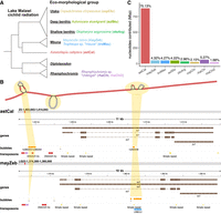
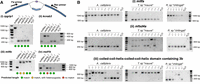
Features of the Lake Malawi haplochromine cichlid assemblies and pangenome graph. (A) Phylogenetic tree of cichlid species used in this study, shown as part of their ecomorphological groups. (B) Visualization of the pangenome graph around the retinal homeobox 1 (rx1) gene involved in cichlid opsin expression. Structural variants (SVs) are represented as bubbles along the Astatotilapia calliptera fAstCal1.2 backbone, whose segments are colored red. These bubbles are juxtaposed with their corresponding locations on the A. callitpera and Maylandia zebra linear reference genomes, on which gene and transposon annotations are provided. (C) Percentage of sequence in the pangenome contributed from each assembly.

The contig N50 values of the newly sequenced genomes range from 0.6 to 8.4 Mbp, with the PacBio assemblies showing better contiguity than the ONT counterparts. Although the assemblies are not chromosome level, they score well when assessed for genome integrity by BUSCO v5.5.0 with the OrthoDB “actinopterygii_odb10” data set (Manni et al. 2021). An average of 3580 out of the 3640 essential genes for ray-finned fishes (98.4%) were completely matched in the PacBio assemblies, comparable to 3539 (97.2%) for A. calliptera and 3580 (98.4%) for M. zebra, respectively. The ONT assemblies for O. argyrosoma, C. chrysonotus, and R. sp. “chilingali” fared worse, with 3406 (93.6%), 3366 (92.5%), and 3420 (93.9%) genes detected, which was expected given that they are more fragmented (Supplemental Fig. S1). Nevertheless, these BUSCO scores suggest that our assemblies exhibit overall good integrity when measured by gene completeness. We also observed little overlap misses between them, with only 30 (0.82%) BUSCOs undetected in more than five assemblies (Supplemental Fig. S1). Together, the eight assemblies represent all but one (Diplotaxodon) of the six major ecomorphological groups of Lake Malawi cichlids, allowing a good baseline sampling of the genomic information in the Lake Malawi radiation.

We utilized the minigraph package to construct a pangenome graph from the Lake Malawi haplochromine cichlid assemblies; minigraph successively adds new genome sequences to the graph structure by a genome-to-graph alignment, starting from a reference genome assembly, known as the backbone (Li et al. 2020). Bubbles are augmented onto the existing graph to represent regions where the new assembly differs sufficiently in sequence from all those already incorporated. We chose the A. calliptera (astCal) genome as the backbone because it is the most contiguous assembly with Ensembl gene annotations available, allowing us to define where SVs are positioned relative to known genes. The remaining assemblies were incorporated in the following order, prioritizing phylogenetic proximity and genome quality: M. zebra (mayZeb), Tropheops sp. “mauve” (troMau), A. stuartgranti (aulStu), O. argyrosoma (otoArg), C. chrysonotus (copChr), and the two Rhamphochromis sp. “chilingali” (rhaChi, rhaChi2).

Structure of the Lake Malawi cichlid pangenome graph

The Lake Malawi cichlid multiassembly graph consisted of linear structures representing the backbone scaffolds, punctuated by bubbles representing SVs (Fig. 1B). Overall, the graph contains 1.171 Gbp distributed across 637,237 segments connected by 913,087 edges. On average, a segment measured 1,839.04 nucleotides in length and was connected by 1.43 edges. The linear part of the graph comprised 189,197 segments containing 758.85 Mbp (64.8% of the total), whereas the variable part (bubbles) was made of 448,040 segments containing 413.05 Mbp (35.2%). As the query assemblies were incorporated, the graph showed greater complexity with increases in the number of edges and segments, accompanied by a decrease in the average length of segments (Supplemental Fig. S2). The backbone-guided nature of graph construction in minigraph meant that the majority of the graph segments originated from the A. calliptera backbone, whose 880,428,986 nucleotides were encompassed within 382,935 segments (Fig. 1C). Incrementally incorporating the other assemblies grew the reference graph by the corresponding number of segments: mayZeb (62,307), troMau (40,627), aulStu (44,206), otoArg (29,209), copChr (21,444), rhaChi (40,742), and rhaChi2 (15,767). These segments consisted of varying number of nucleotides: mayZeb (50,651,908), troMau (50,003,806), aulStu (49,458,672), otoArg (34,661,015), copChr (25,161,891), rhaChi (61,804,019), and rhaChi2 (19,731,824). The query assemblies contributed a cumulative total of 291.47 Mbp, or 33.1%, additional nucleotides compared with the A. calliptera backbone. These nonreference sequences were encapsulated within a total of 188,944 bubbles, positioned in backbone regions that span the structural breakpoints from at least one of the nonreference samples. Out of the 880,428,986 nucleotides on the backbone segments, a substantial 840,567,200 (95.47%) received spanning coverage (Supplemental Figs. S3, S4), which translates to a bubble density of 0.2248 per 1 kbp of covered backbone sequence.

The construction of a multiassembly graph with minigraph relies on the initial choice of a backbone assembly, and it has been reported that this could directly impact the amount of nonreference sequence that is detected from the subsequent assemblies (Crysnanto et al. 2021). To investigate the robustness of our multiassembly graph, we built seven other graphs using each of the nonreference samples as the backbone in turn. The more contiguous PacBio backbones produced graphs that were topologically more complex than their ONT counterparts with larger number of segments, edges, bubbles, and extra sequence. Nevertheless, the proportions of linear and variable sequences were similar across all the backbones at ∼65% and ∼35%, respectively (Supplemental Fig. S5), whereas most metrics in the PacBio-based graphs fell within 5% of those of the canonical A. calliptera version (Supplemental Table S1). Permuting the order of incorporation of the subsequent assemblies did not significantly affect graph structure and topology, suggesting that backbone choice was the dominant factor in the variation that was observed (Supplemental Fig. S6). For a fair comparison of bubble frequency, we normalized the bubble counts by the number of backbone nucleotides with spanning coverage, and found that these values ranged from 0.2192 to 0.2254 bubbles per kilobase pair of covered genomic sequence (A. calliptera, 0.2248). These observations suggest that minigraph is consistent for SV discovery and that the default graph exhibits a reasonable structure and amount of sequence information.

Finally, we examined how multiassembly graph construction behaved in response to the choice of the minimum variant length (L) in minigraph, which influences the minimum length of sequence difference required for a bubble to be created. We utilized the default value of L = 50, as it follows the conventional definition of a SV. This has the advantage of ignoring smaller-scale variation (SNPs, small indels) and making the graph less complex and more interpretable, which is appropriate for the focus on larger-scale variation in this study. Although the topological complexity of the multiassembly graph decreases with larger values of L, we found that there was a relatively broad parameter range of L = 25 to 500 at which the total sequence content in the reference graph remained relatively stable (Supplemental Fig. S7; Supplemental Table S2).

Substantial proportion of nonreference sequences in the pangenome

The majority of SV sequences in the graph bubbles of the Lake Malawi cichlid pangenome originated from nonreference assemblies rather than the backbone (Fig. 2A). The amount of sequence from the seven other assemblies totaled up to 291.47 Mbp, or 33.1% of the size of the A. calliptera backbone, averaging to a median of 49.46 Mbp per assembly. Conversely, the amount of A. calliptera backbone sequence located within bubbles was lower at ∼13.81%, or 121.57 Mbp. Repeating this analysis across the graphs with different backbones also showed a similar pattern in which more of the uncovered SV sequences were attributed to nonreference sequences rather than the backbone (Supplemental Fig. S8). This suggests that each assembly contains stretches of genomic sequences that might have been overlooked if we had only focused on any individual backbone as a reference, highlighting the value of the pangenome approach.

View larger version:

• In this window
• In a new window

• Download as PowerPoint Slide

Figure 2.

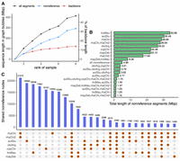
Nonreference sequences in Lake Malawi pangenome graph. (A) Length of SV sequences in the graph bubbles, based on whether they originated from nonreference assemblies (blue) or the backbone (red). (B,C) Cumulative length and number of graph segments shared across assemblies.

Following this, we uncovered that the nonreference sequences in the pangenome did not originate from a single assembly, but instead, similar amounts were contributed by the seven genomes. The majority of nonreference graph segments containing the SV sequences were only present in one genome, making them singletons or private variation (Fig. 2B,C). These cumulatively account for 182.16 (62.5%) out of 291.47 Mbp spread across 115,173 (45.3%) out of the 254,201 nonreference segments within the bubbles. Notably, the higher-quality PacBio assemblies contributed the most unique sequences to the pangenome: troMau (33.98 Mbp), aulStu (30.49 Mbp), and rhaChi (28.99 Mbp). However, we also observed some degree of sequence common between the genomes (Fig. 2B,C), the greatest amount of which was between the two Rhamphochromis (28.09 Mbp shared across 21,272 segments). Finally, there was 4.98 Mbp of sequence detectable in all the nonreference assemblies but absent from A. calliptera. These bubbles instead contained a substantial amount of backbone sequences that were private to the A. calliptera assembly: 22,511 segments harboring 42.32 Mbp (4.81% of the backbone). These results suggest that the SV landscape of the Lake Malawi cichlids is dominated by singletons.

Discovery of SVs

We investigated the 188,452 bubbles in the reference graph in detail and found that the majority harbored straightforward presence-or-absence variation or slightly nested variation, with complex structural variation being relatively rare (Supplemental Fig. S9). The number of possible paths to traverse a bubble exhibited a strongly left skewed distribution toward simple variation: There were 151,761 (81%) two-path and 21,230 (11%) three-path bubbles, and 182,136 (97%) had no more than eight theoretical paths (Supplemental Fig. S10). To focus on true biological variation within the bubbles, or the alleles, we retain only the paths actually transversed by samples. Using minigraph, we were able to successfully call alleles for all samples at 160,578 out of the 188,452 bubbles (85.2%). For subsequent analyses, we retained 187,552 out of the 188,452 bubbles (99.5%) for which the alleles are known for at least five out of eight samples to facilitate between-sample comparisons (Supplemental Fig. S11).

Most of the retained bubbles were biallelic (153,848, 82%), whereas the remaining multiallelic ones mostly contained three alleles (20,751, 11%). The graph was composed of mostly simple structural variation, many of which were singletons (Fig. 3A), but the size of the SVs varied widely. A total of 434,357 alleles were observed across the 187,552 bubbles, which translated to an average of 2.32 alleles per bubble. The 246,805 nonreference alleles in this set comprised 144,769 insertions, 101,179 deletions, and 857 substitutions/inversions with an average length of 2016.7, 1510.8, and 605.2 bases, respectively (Fig. 3B). The cumulative length of insertions was 291.96 Mbp, which was longer than the 152.86 Mbp associated with deletions. The length of SVs shows a peak above 1000 bp, with the top 1% longest insertions ranging from 17,469 to 251,778 bp and deletions measuring 19,567 to 215,374 bp. The Lake Malawi cichlid multiassembly graph contained more complete insertions (78,479; only nonreference allele with sequence, reference length of zero) compared with partial/alternate insertions (66,290; both reference and nonreference sequences present, but the nonreference allele is longer). We observed the opposite pattern with deletions: 49,217 complete versus 51,962 partial/alternate.

View larger version:

• In this window
• In a new window

• Download as PowerPoint Slide

Figure 3.

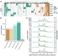
The Lake Malawi cichlid SV landscape. (A) Heatmap showing length difference of alleles for each nonreference sample versus the A. calliptera backbone across 5000 random bubbles, shown as columns. A positive value (green) represents an insertion, and a negative value (brown) represents a deletion, with darker colors indicating larger SVs/indels. (B) Number of SV alleles by type. (C) Length deviations of nonreference alleles across different sample frequencies. Dashed line denotes 50 bp.

Most of the biological alleles in the reference graph are single insertion or deletion events that are present at a low sample frequency across our eight assemblies. A significant majority of alleles (147,802 or 60%) are singletons, meaning that the nonreference allele had a sample frequency of either one out of eight (135,160 alleles), or seven out of eight (12,642 alleles), in which case the reference allele on the A. calliptera backbone is the singleton (Fig. 3C). These results are consistent with the observation in the previous section that many nonreference segments and sequences are private to a single assembly (Fig. 2). The extreme sample frequencies were primarily dominated by the large SVs measuring thousands of base pairs in length, with one of eight and two of eight frequencies dominated by complete insertions and seven of eight by complete deletions (i.e., complete insertions in A. calliptera backbone relative to the others). Conversely, intermediate allele frequencies tended to be composed of shorter sequence variants, with most having a length of ∼50 bp (Fig. 3C).

Recapitulation of species relationships

We investigated how the phylogenetic information in the multiassembly graph compares to what is known about species relationships from SNP studies of the Lake Malawi cichlid radiation (Malinsky et al. 2018). Overall, the pangenome graph closely reflected the expected interspecies relationships based on the prevailing understanding of the evolutionary history of the Lake Malawi cichlid radiation (Fig. 1A), despite the fact that the assemblies varied in their quality and the sequencing technologies used. For instance, we successfully recapitulated known cichlid groupings in a principal component analysis (PCA) plot based on a presence/absence matrix across the 150,532 bubbles containing two or three observed alleles (Fig. 4A). Using this same presence/absence matrix, we also constructed a phylogenetic tree based on the number of SV events between samples (Fig. 4B), revealing a median of 56,402 differences. We also observed a considerable amount of interspecies polymorphism, with the highest levels between the mbuna species Tropheops sp. “mauve” and M. zebra, which shared 111,695 events (74.2%). The two Rhamphochromis individuals shared 124,364 (82.6%), while also showing higher correlation of SV lengths and differing allele sequences at noticeably fewer positions (Supplemental Fig. S12).

View larger version:

• In this window
• In a new window

• Download as PowerPoint Slide

Figure 4.

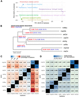
Estimation of phylogenetic relationships between Lake Malawi cichlid assemblies. (A) Principal component analysis of the samples based on a presence/absence matrix across 150,532 bubbles with at most three alleles. (B) Midpoint-rooted neighbor joining tree of Malawi samples estimated from SV events. The distance between any two samples corresponds to the total horizontal branch length separating them. Nodes are labeled with the number of sites at which descendant samples share the same allele (first number) and inserted sequences relative to the shortest allele observed across all samples (second number). (C,D) Structural variation manifested between biassembly graphs between sample pairs as a percentage or bubble density. Comparisons are asymmetrical, in which one assembly acts as a backbone against which the other query is aligned. Minimum variant size in minigraph was set to 50.

Next, we constructed biassembly graphs from every possible pair of samples to perform a one-to-one estimation of the sequence that manifests as SVs between them. This was intended to complement previous estimates of 0.1% to 0.25% pairwise SNP divergence in Lake Malawi cichlids. Unlike SNP studies, this comparison is asymmetrical, in which one assembly acts as a backbone and the other as a query, from which the SV percentage is estimated as the percentage of backbone regions within bubbles (Fig. 4C). With the default minimum variant length parameter L = 50 and correcting for sequencing coverage, estimated interspecies SV proportion ranged from 4.73% to 9.86% (mean, 7.11%), with smaller values within the mbuna (mean, 5.45%) and benthic (mean, 5.20%) groups. The estimated differences were much lower within species when comparing the two Rhamphochromis individuals (2.96% and 3.68%). We tested parameter values of L from 2 to 250 and found that these estimated percentage differences were representative of those at larger L values, as smaller variants and potential sequencing errors in the assemblies were gradually excluded (Supplemental Fig. S13).

Using these same biassembly graphs, we next obtained a measure of how frequently structural events occur along the genome by calculating the bubble density normalized by spanning coverage (Fig. 4D). This revealed an interspecies bubble density of 0.061 to 0.098 per 1 kbp of backbone compared with an intraspecies density of 0.041 among the two Rhamphochromis. There appeared to be some directionality to the sequence changes, as both Rhamphochromis individuals contained more insertions and fewer deletions when aligned to the other species (Supplemental Fig. S14). This high similarity between the two Rhamphochromis individuals is expected as they belong to the same species and might have exhibited structural changes independently of the other cichlids. This is consistent with the SNP-based Lake Malawi cichlid phylogeny in which the pelagic group that contains the Rhamphochromis and Diplotaxodon taxa branched off earlier than the rest of the radiation (Fig. 1A).

PCR validation and genotyping

We performed polymerase chain reaction (PCR) validation of 16 predicted SVs, using five of the original tissue samples that were used for genome sequencing of troMau, otoArg, copChr, rhaChi, and rhaChi2. Because of difficulties in designing PCR primers for repetitive genomic regions, we prioritized bubbles containing simple, straightforward presence-or-absence variants located within 1500 bp of a gene. Out of the bubbles we tested, the validation results for 12 were consistent with the allele predictions for all five assemblies, whereas the remaining four matched the allele predictions of four assemblies (Fig. 5A; Supplemental Table S3). Some heterozygosity was present in four of the 12 bubbles, which was expected because our samples were not from homozygous lines. At such heterozygous sites, allelic information across parental chromosomes would have been collapsed into a single sequence, showing only one of two alleles in the assembly. Ten out of 16 SV PCR results were further verified by Sanger sequencing (Supplemental Table S3). For the remaining six out of 16 SVs, PCR results were partially validated by Sanger sequencing, as we could not acquire good quality sequencing in some instances, likely because of the repetitive nature of these loci. However, all sequenced PCR products that were obtained corresponded to the expected sequences. Overall, these results provide additional experimental support to our findings and demonstrate the reliability of SV detection with minigraph.

View larger version:

• In this window
• In a new window

• Download as PowerPoint Slide

Figure 5.

PCR genotyping of SVs. (A) Validation of predicted SVs in original samples. Green indicates match; amber, match with heterozygosity; and red, no match. (B) Wider genotyping across aquarium-grown individuals: 10 A. calliptera (five males, five females), nine Tropheops males, and six Rhamphochromis (one male, five females).

We also utilized the designed PCR primers to perform additional genotyping of a wider cohort of aquarium-reared male and female individuals of A. calliptera, Tropheops sp. “mauve” and Rhamphochromis sp. “chilingali” to check for evidence of polymorphism at some bubbles (Fig. 5B). For example, we did not find any evidence for polymorphism in a bubble near mitfa (ENSACLG00000022427), with all genotyped A. calliptera and Rhamphochromis sp. “chilingali” showing one allele and all Tropheops sp. “mauve” showing the other. However, bubbles near some genes (mfsd4a and ENSACLG00000002767) showed evidence of polymorphism in different sexes and species. These observations suggest a variable degree of SV polymorphism and heterozygosity in Lake Malawi cichlids. However, there is limited statistical power to draw any conclusions about the wider Lake Malawi cichlid radiation given our small sample sizes.

SVs are underrepresented in protein-coding regions

To investigate the functional relevance of the SVs, we examined the 187,552 bubbles for the presence of nearby genes. We focused on a subset of 26,734 out of 28,001 gene annotations in the A. calliptera genome, filtering out putative TEs misannotated as genes (see Methods); 90,531 (48.3%) bubbles directly intersected with genic features like exons, introns, or UTRs, whereas 8967 (4.8%) and 6010 (3.2%) were located within 2000 bp upstream of and downstream from genes, respectively. The remaining 82,024 (43.7%) were considered intergenic, located an average of 38.4 kbp from the nearest gene start. Coverage-corrected bubble densities were 0.2481 per kilobase pair of intergenic sequence and 0.2213 for introns, similar to the genome-wide level of 0.2248, but the bubble density in exonic regions was significantly lower at 0.0899 per kilobase pair (Fig. 6A). Functional enrichment analysis found that genes containing SVs are associated with broad Gene Ontology categories, including transport (P-value = 2.122 × 10⁻³³), phosphorus metabolic process (P-value = 6.204 × 10⁻²³), and developmental process (P-value = 5.660 × 10⁻²¹) (Supplemental Fig. S15). The transport and phosphorus metabolic process categories include potassium channels and bone morphogenetic proteins, whereas the developmental process involves forkhead box (FOX) genes and fibroblast growth factor receptor 1. There were 4723 (17.7%) genes in which SVs were entirely absent from the gene body and within a 2000 bp region, which we consider a highly conserved set of genes across species. This gene set was associated with terms related to transcription and translation: gene expression (P-value = 4.4 × 10⁻⁴⁰), RNA-induced silencing complex (RISC) (P-value = 9.2 × 10⁻³⁸), DNA-binding transcription factor activity (P-value = 1.6 × 10⁻¹³), and structural component of ribosome (P-value = 1.9 × 10⁻¹⁰) (Supplemental Fig. S16).

View larger version:

• In this window
• In a new window

• Download as PowerPoint Slide

Figure 6.

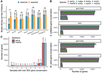
Genomic context of SVs. (A) Bubble density in gene features; 95% confidence intervals are estimated across 100 bootstraps, for which the SV coordinates were shuffled within ±1000 bp of their original positions (observed) or randomly across the whole genome (expected). (***) P-value < 1 × 10⁻³, (n.s.) not significant. (B) Percentage sequence conservation of genes calculated for backbones with gene annotations. (C) Presence–absence counts of backbone genes. A value of one denotes genes that are not detectable in the other assemblies and might be private, and a value of eight refers to ubiquitous genes.

Subsequently, we estimated the percentage conservation of genes for each sample based on the path they traversed through the graph. This calculation was performed for a set of 20,785 (86.9%) genes on the A. calliptera–backboned graph, which were located outside overly complex bubbles and had spanning coverage from all samples. This approach suggested that 83.2% to 85.6% of genes showed >95% sequence conservation in the gene body across the nonbackbone samples, with ecologically similar species exhibiting similar percentage conservation scores to each other (Fig. 6B). This conservation was more pronounced in exonic regions, where 93.5% to 94.7% of genes maintained this high level of conservation. We observed similar patterns with the corresponding set of 20,266 (85.6%) M. zebra genes, suggesting this high sequence conservation was robust against reference bias (Supplemental Table S4).

We counted the presence of each gene across the eight assemblies, applying a lenient 50% conservation threshold to accommodate large introns. This analysis covered a larger set of 24,322 (86.9%) A. calliptera and 24,532 (85.6%) M. zebra genes within regions that had spanning coverage from at least six samples. As expected, a large proportion of genes—21,407 (88.0%) A. calliptera and 20,964 (85.5%) M. zebra—was detectable in the other assemblies. This approach indicated that A. calliptera and M. zebra had 378 and 260 gene sequences that were unique relative to the other assemblies (Fig. 6C). These genes contain protein domains that are ubiquitous and multicopy across eukaryotic protein families (Supplemental Fig. S17), including ubiquitin-like, zinc-fingers, ankyrin repeats, and G protein–coupled receptor (GPCR) domains. However, a TBLASTN search suggested that these were likely false positives: 365 (96.6%) supposedly unique A. calliptera genes were detectable in M. zebra, and 219 (84.2%) vice versa. For instance, several hemoglobin genes thought to be private to the A. calliptera were traced to assembly errors that caused the formation of artifact bubbles in the pangenome graph (Supplemental Fig. S18). Overall, the available evidence suggests that the sequence differences between Lake Malawi cichlids are unlikely to be caused by preferential gene gain or loss in certain groups.

Enrichment of TEs in SVs

Having observed that most of the SVs do not occur in protein-coding regions of genes, we turned our attention to TEs, which have been shown to be sources of phenotypic novelty in cichlid fishes (Santos et al. 2014; Carleton et al. 2020; Munby et al. 2021). About 36.55% of the A. calliptera sequences are annotated by RepeatModeler/RepeatMasker as TEs, of which the biggest classes were DNA transposons (12.09%), LINEs (8.32%), and LTR retrotransposons (7.38%), whereas the SINEs, helitrons, and retroposons collectively take up <1% (Fig. 7A). There is also a substantial number of unknown elements (8.54%), which might constitute currently uncharacterized TEs and other repetitive elements. Overlap analysis suggested that 74.65% of SVs sequences on the backbone were annotated as TEs, which is a 2.04-fold increase compared with genome-wide TE distribution, or 2.20-fold if unknown elements were excluded (62.25% TEs). This enrichment was still detectable even when SV coordinates were randomized and were across varying sequence divergence thresholds for TE detection in RepeatMasker, with the DNA, LINE, and LTR transposons consistently showing strong enrichment (Supplemental Fig. S19; Supplemental Table S5). These genome-wide and SV transposon proportions were also reflected in the other species, ranging from 36.32% to 38.29% genome-wide and 72.26% to 75.74% in SVs, suggesting that TEs represent most of the large-scale sequence differences among the cichlid assemblies (Supplemental Table S6).

View larger version:

• In this window
• In a new window

• Download as PowerPoint Slide

Figure 7.

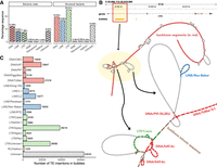
Transposable elements (TEs) in the Lake Malawi cichlid pangenome. (A) Genome-wide and SV TE composition of the A. calliptera fAstCal1.2 assembly. (B) TE insertions in the first intron of mitfa, highlighting the presence of two complex bubbles. (C) Number of putative polymorphic TE insertion events by subclass across 90,451 bubbles.

Closer inspection showed that the multiassembly graph successfully incorporated known examples of SV/TEs in Lake Malawi cichlids, such as a haplochromine-specific SINE insertion upstream of fhl2b important for egg spot patterning (Supplemental Fig. S20; Santos et al. 2014), as well as a nested insertion upstream of rx1 whose alleles contribute to different opsin palettes in cichlid vision (Supplemental Fig. S21; Schulte et al. 2014). Another example is the mitfa gene, whose first intron harbors the presence of complex variation caused by TE insertions (Fig. 7B), consistent with previous observations (Carleton et al. 2020). Although we refrain from making claims about species-level differences in TE composition, owing to the varying quality of the assemblies, we performed a high-level characterization of the subclasses of TEs within graph bubbles as they might indicate classes that are still segregating within the Lake Malawi population. By overlapping TE coordinates against SVs across all the assemblies, we identified 254,015 straightforward presence-or-absence TE insertion events across 90,451 unique bubbles (Fig. 7C). The most frequent within-bubble TE insertions involved the subclasses of LTR/Gypsy (38,216), LTR/Unknown (28,080), DNA/TcMar (21,518), DNA/hAT (18,947) LINE/Rex-Babar (18,292), and LINE/L2 (13,077). On a genome-wide scale, 14,868 genes (55.9%) had a putative polymorphic TE bubble in the gene body or within 2000 bp upstream. This number decreased to 7898 (29.7%) if we required the bubble to be in proximity to the start of the gene. None of these intersections revealed a significant Gene Ontology enrichment, even when stratifying for TE classes and subclasses. This lack of functional enrichment supports the hypothesis that species-variable TE insertions display no apparent pattern or preference for specific genes.