
Abstract
Meiosis relies on programmed DNA double-strand breaks (DSBs) to initiate recombination between homologous chromosomes. Only a fraction of these breaks mature into crossovers (COs), creating the chiasmata essential for physically linking homologs and ensuring their accurate segregation in meiosis I. Errors in CO number or placement underlie a large fraction of human infertility and aneuploidies, yet how DSBs are designated to become COs and how the mechanisms ensuring COs form on all chromosomes (CO assurance) are not well understood, particularly in systems with a large number of chromosomes. Here, we investigate CO formation in the pantry moth, Plodia interpunctella, a novel invertebrate model system with n = 31 chromosomes. Using a combination of sequencing approaches, Oligopaints FISH, and statistical Weinstein tetrad analysis, we find robust CO assurance and interference in Plodia, with most chromosomes harboring only a single distal CO and few bivalents lacking COs. We employ CUT&RUN, ATAC-seq, and RNA-seq to profile the epigenomic landscape in Plodia testes, revealing that the distal chromosome arms in which COs form are enriched for heterochromatin and devoid of accessible chromatin, suggesting a bias for COs to form in repressed regions in the genome. These studies pave the way for future work diving deeper into the molecular regulation of CO formation in Plodia and other systems, in which the large number of chromosomes may be the key to revealing novel insights about CO regulation.
Meiosis is the specialized cell division that occurs in the germline to produce haploid gametes. Once cells enter meiosis, maternal and paternal chromosome copies come together for pairing and meiotic recombination, also known as crossing over. In addition to generating genetic diversity, in most species, crossover (CO) formation also serves the key function of linking maternal and paternal homologs until they are segregated at anaphase I. This link between homologs not only prevents their premature separation but also is required for proper chromosome alignment and kinetochore tension at metaphase I (Nicklas 1997; Davis and Smith 2003; Nambiar et al. 2019). The accurate regulation of these chromosome dynamics during meiosis I is essential for the formation of healthy, viable gametes and failure to do so can result in chromosomal disorders or infertility (Bolcun-Filas and Handel 2018). In humans, many meiotic errors occur during these early stages of meiosis I as the result of defects in the number or placement of COs (Martin 2006; Sun et al. 2007a,b).
Crossing over begins with the formation of programmed DNA double-strand breaks (DSBs), a subset of which are repaired as COs (Gray and Cohen 2016). In most species, far more DNA DSBs form than COs (de Massy 2013), and most DSBs are repaired as non-CO events. How DSBs are designated into CO or non-CO repair is still a major question in the field. What is clear is that CO formation is very tightly regulated and governed by many “rules.” First, CO assurance is a meiotic regulatory principle that ensures each homologous pair gets at least one CO to link them together (Darlington and Dark 1932; Owen 1949). Second, COs have a reduced likelihood of forming between adjacent regions of the same chromosome owing to CO interference (Sturtevant 1915; Muller 1916; Otto and Payseur 2019). Apart from yeast, systems with small chromosomes almost always have only one or two COs per chromosome owing to CO interference. Finally, COs are unlikely to form in chromosome regions required for genome stability, such as centromeres, which is known as the “centromere effect” (for review, see Saito and Colaiácovo 2017; Pazhayam et al. 2021).
Despite these widely observed rules, the factors that regulate CO formation and designation are highly diverse in sequence and function across species (Gerton and Hawley 2005; Kumar et al. 2010; Keeney et al. 2014; Dapper and Payseur 2019; Arter and Keeney 2024). As a result, CO locations vary across eukaryotes, even between closely related species (Price and Bantock 1975; Stapley et al. 2017; Samuk et al. 2020). The position and distribution of COs can even differ between individuals of the same species, such as differences in CO landscapes between males and females, called heterochiasmy (Lenormand and Dutheil 2005; Kong et al. 2014; Theodosiou et al. 2016; Brekke et al. 2023). Finally, CO placement can be altered owing to environmental factors such as temperature, infection status, and oxidative stress (Bomblies et al. 2015; Rybnikov et al. 2023).
The causes and consequences of this plasticity in CO formation are unclear, as are the mechanisms regulating CO assurance and interference. How does each cell ensure that all chromosomes get a CO? How does the formation of one CO prevent the formation of neighboring COs? Here, we employ the pantry moth, Plodia interpunctella, as a novel model system for interrogating CO formation. This study aims to broaden our analyses of meiotic recombination to include emerging systems such as Plodia, which is essential for revealing the true breadth of meiotic recombination strategies.
Results
Whole-genome sequencing of two laboratory strains of Plodia reveals genetic variation within and between strains
To analyze meiotic COs in Plodia, we obtained two divergent laboratory strains of P. interpunctella: the Savannah strain and the bFog strain (Fig. 1A). The Savannah strain originated as a wild strain isolated in Savannah, Georgia, and has been inbred in U.S. Department of Agriculture (USDA) laboratories since the late 1960s (Lum and Flaherty 1970). The bFog strain is a newer laboratory strain that was generated only a few years ago as a hybrid between two additional, independently isolated wild strains: the Dundee, United Kingdom, and the Florida laboratory strains (Heryanto et al. 2022). To map COs between chromosomes of these two strains, we first needed to identify all the genomic variants between these strains. For this, we performed whole-genome Illumina sequencing on three individuals per strain to generate genome-wide variant (SNP) maps. Because these are not isogenic strains and Plodia have not been inbred for as long as other laboratory systems like Drosophila, we were able to capture both interstrain variants and intrastrain variants using this approach.
Genetic variation in Plodia strains. (A) Image of the adult female Plodia interpunctella strains used in this study: the bFog strain (left) and the Savannah strain (right). (B) Number of variants per chromosome between individuals in our bFog (red) and Savannah (blue) strains. The plot shows the count of variants across three WT individuals for each strain. An intrastrain variant is a single–base pair locus that is different between any of the individuals. (C) Plots showing the position and enrichment of intrastrain variants on individual chromosomes for the bFog strain (left) and Savannah strain (right). (D) Histogram showing the minimum distance of identified strain-specific variants from the end of a chromosome, in which the number of variants for each chromosome is binned using 30 kb windows. The genome was subdivided into three chromosome-sized groups, with Chr 1–10 (largest; 12.65–10.82 Mb) shown here. The “skewness” of variants toward the chromosome end is as follows for Chr 1–10: Savannah = 0.157 and bFog = 0.276. Dashed lines show the mid-point of the smallest chromosome per chromosome group, and solid lines show the mid-point of the largest chromosome per chromosome group. (E) Representative structural variants (blue) detected in the genome of our Savannah strain individuals compared with the reference Plodia Savannah genome. (F) Haplotype-specific variants per chromosome in the bFog (red) and Savannah (blue) strains. (G) Schematic of HOPs for Chr 3 designed based on variants detected in the whole-genome sequencing data. (H–J) Chr 3 HOPs FISH on mitotic germline stem cell (H), pachytene cell (I), and diakinesis cell (J) from male F1 hybrids testes squashes. DAPI is shown in gray, bFog Chr 3 in red, Savannah (Sav) Chr 3 in blue, and Chr 11 control in yellow.
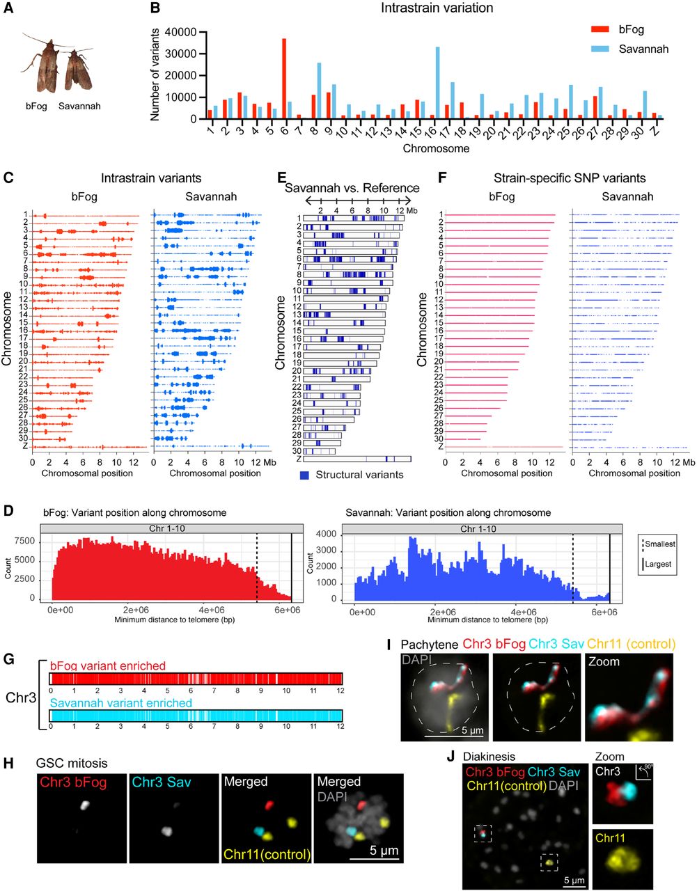
Significant variation was observed both between the two strains and among the three individuals of each strain. Overall, the Savannah strain showed more intrastrain SNP variation than the bFog strain, with one Savannah individual being particularly different from the other two. We found this high variation within the Savannah strain quite surprising, because this strain has been inbred in laboratory cultures for >50 years. Among the three individuals per strain, the Savannah strain had more SNP variants on Chr 8 and 16, whereas bFog had more variants on Chr 6. Chr 7, along with the Z sex chromosome, had the smallest number of identified variants in both strains (Fig. 1B,C). These identified intrastrain variants (defined as any one individual harboring a distinct allele at that locus) were broadly distributed in clusters across chromosomes, with a few exceptions in which variants were more localized. For example, Savannah Chr 11 only had observed variants along one arm (we define “arms” as the distal thirds of a chromosome), and bFog Chr 2 and 9 harbored pockets of variants toward chromosome centers (Fig. 1C). In general, the identified bFog variants tended to be slightly closer to chromosome ends, whereas Savannah variants had less positional skew (Fig. 1D; Supplemental Fig. S1; Supplemental Table S1).
In agreement with the observed intrastrain SNP variation detected using Illumina sequencing, we also performed Pacific Biosciences (PacBio) long-read sequencing on three additional individuals per strain. Using the PacBio data, we identified many structural variants (insertions, deletions, or translocations) that were common to all three sequenced individuals of our Savannah stock compared with the reference Plodia genome generated from Savannah moths (Fig. 1E). However, it is worth noting that we did not perform Hi-C or other supplemental scaffolding approaches to verify this.
When comparing SNPs between the Savannah and bFog strains, we only considered alleles that were consistent between all three individuals of a strain and differed between strains. Using this method, we detected enough SNPs for accurate breakpoint detection in our data every 50–75 bp (Fig. 1F). To validate these strain-specific SNPs, we designed haplotype-specific Oligopaints (HOPs) (Beliveau et al. 2015; AlHaj Abed et al. 2019) for Chr 3 (Fig. 1G). These paints should exclusively label either the bFog Chr 3 or Savannah Chr 3 alleles, resulting in two nonoverlapping FISH signals for Chr 3 in hybrids. We tested these HOPs in cells with both paired and unpaired chromosomes in testes from first-generation (F1) hybrids. We indeed observed two distinct FISH signals for Chr 3 (Fig. 1H–J). Notably, there are fewer variants toward the middle of Chr 3 for both strains (Fig. 1C,F,G), resulting in weaker FISH signals toward chromosome centers (in which there are fewer probes per kilobase). This is especially obvious when the chromosomes are in a linear configuration like at pachytene (Fig. 1I).
As a possible explanation for the genetic variation in our strains, we investigated repetitive DNA content in the Plodia genome. Repetitive sequences such as transposable elements (TEs) are often rapidly evolving owing to a lack of selective pressure at these loci (Finnegan 1989; Gbadegesin 2012; Lawlor and Ellison 2023). Using repeat modeling and annotation of the reference Plodia assembly, we identified several repetitive sequences likely belonging to TEs, which overall represent 18% of the Plodia genome (Supplemental Fig. S2A). Of all identified TEs, ∼9% are SINE-like, ∼30% are LINE-like, ∼15% are LTR-like, 6.5% are DNA transposons, and ∼40% are rolling circle (RC) repeats (Supplemental Fig. S2A). The relatively high representation of RCs, comprising ∼7% of the Plodia genome, is consistent with the broad range of RC abundances reported in Lepidoptera, in which considerable heterogeneity in RC content has been observed among species (Baril and Hayward 2022; Zhang et al. 2023; Perrier et al. 2025).
Repeat modeling performed on our strain-specific PacBio sequencing data also led to the identification of a potential satellite sequence with high sequence similarity between the bFog and Savannah strains, which is also present in the reference Plodia assembly (Supplemental Fig. S2B). Although this potential satellite sequence does not show any specific accumulation in chromosome arms versus centers, the majority of the TEs are found in the two distal arm regions of chromosomes genome-wide, except for small chromosomes in which TEs are more evenly distributed (Supplemental Figs. S3A, S4A; Supplemental Data Set S1).
We tested whether strain-specific variants are enriched within these TEs, and we found that, indeed, variants are significantly enriched in TEs, but the odds ratios are low (1.2 for Savannah and 1.18 for bFog, Fisher's exact test). (Supplemental Fig. S3A,B; Supplemental Data Set S2; Supplemental File S1). If variants are more likely to accumulate in repetitive elements, then perhaps they are excluded from coding regions like gene bodies. When we tested whether variants are excluded from gene bodies or not, we found that, yes, both of the Savannah and bFog variants are significantly depleted from gene bodies but, again, with mild odds ratios (0.86 and 0.92, respectively). In summary, variants are somewhat enriched in TEs and excluded from gene bodies, but the biological significance of this is unclear. Regardless of the underlying mechanism, the variations we detected using this genome sequencing approach suggest that the Plodia genome is not necessarily under strong purifying selection and may even have regions that are quickly evolving.
CO analysis in Plodia reveals strong CO assurance and interference
Having identified genome-wide, strain-specific variants in our wild-type parental strains (WTs), we needed to generate hybrids to map COs. As only male meiosis is reported to involve COs in Lepidoptera (Rasmussen 1977; Rasmussen and Holm 1982; Xiang et al. 2024), we isolated hybrid males (F1s) which harbor sperm containing CO chromatids. We then crossed these male F1 hybrids back to either WT Savannah or WT bFog females to generate F2 hybrids heterozygous for F1 COs (Fig. 2A). Whole-genome sequencing was performed on these F2s. A detailed description of these crosses can be found in the Methods. As a control, we also generated F2s from F1 hybrid females backcrossed to WT Savannah males (“HFS”), from which we expected to recover no F1 COs (Supplemental Fig. S5A,B).
CO analysis in Plodia. (A) Schematic of crosses to generate hybrids for whole-genome sequencing. bFog chromosome is shown in red and Savannah chromosome in blue. (B) Representative coverage plots of Savannah backcrosses for three chromosomes to visualize CO(s). SNP coverage plots for Chr 18, 13, and 3 showing NoCO, SCO, and DCO, respectively. (Top) SNP density plot and (bottom) chromatids for each chromosome after CO showing chromosome regions from bFog (red) and Savannah (blue), as shown in A. (C) Bar graph showing F2 CO quantification in this study for each chromosomal location of CO chromatids identified in the F2s. NoCO is shown in white, SCO in gray, and DCO in black. (Bottom right) Pie chart showing genome-wide percentage of COs quantified in F2 hybrids. NoCO = 47%, SCO = 50%, and DCO = 3%. (D) Round spermatids labeled with HOPs, with the Savannah allele in cyan and the bFog allele in red. DAPI is shown in blue. (Left) Field of cells; (right) zoom of representative single cells showing NoCO, SCO, or DCO; and (below) quantification percentage for Chr 3 in round spermatids. (E) Quantification of COs present on Chr 3 in round spermatids by FISH compared with F2 sequencing. (F) Coefficient of coincidence (CoC; observed/expected DCO events) versus genetic distance for both Plodia (blue) and Drosophila (green). A CoC value of one indicates no CO interference. (G) Quantification of HEI10 foci number based on immunofluorescence in early prophase I cells from spermatocyte spreads. (Right) Zoom of HEI10 quantification at pachytene. (H) Representative images of HEI10 immunofluorescence in early prophase I cells (leptotene, zygotene, and pachytene).
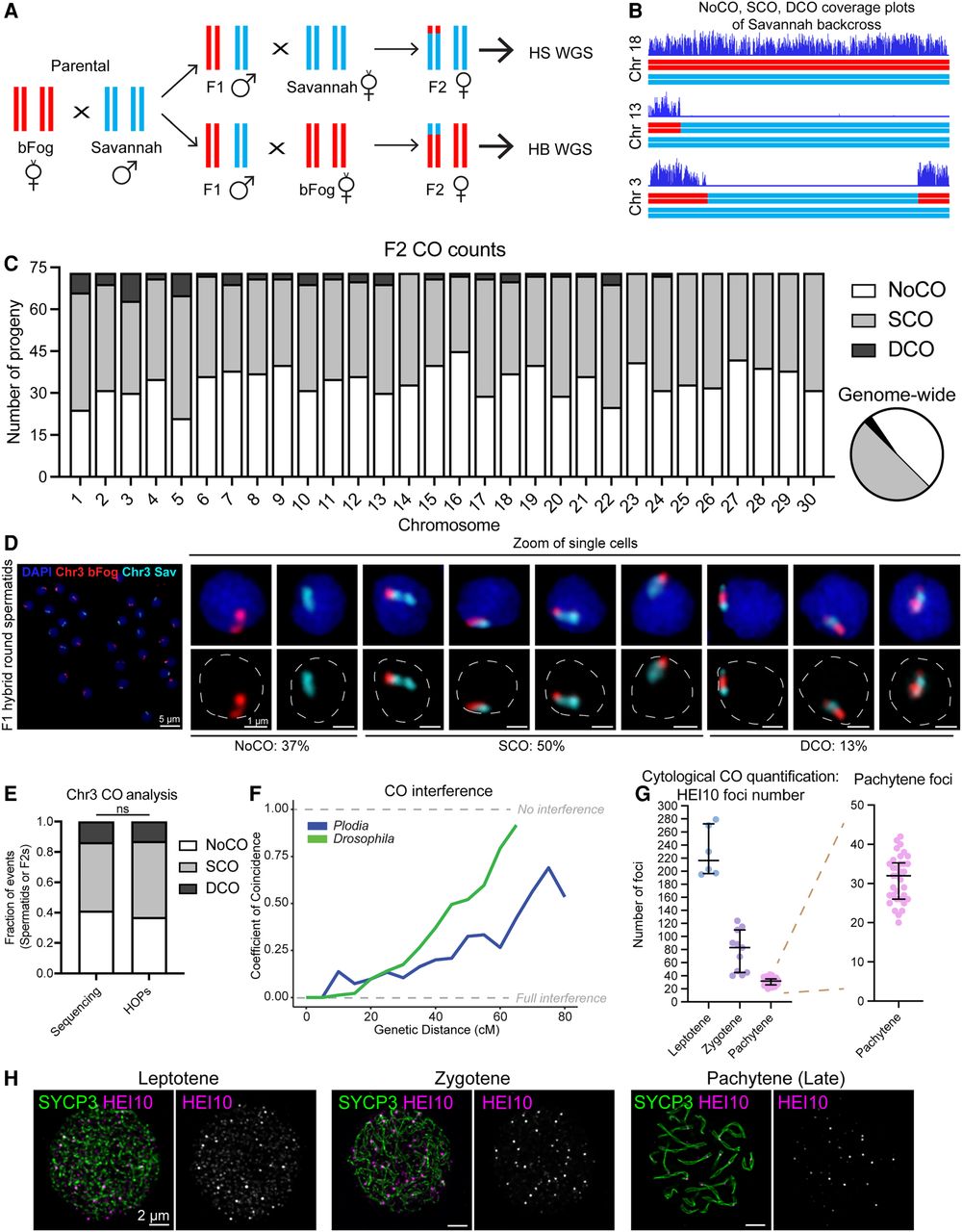
From the genomic DNA of these F2 hybrids, we performed Illumina sequencing, computationally identified strain-specific variants, and performed downstream analysis to detect F1 COs (see Methods). Variants were called relative to the Savannah strain reference genome. Because of the expected greater number of variants from the bFog background, we used different quantification methods for hybrids backcrossed to WT bFog versus WT Savannah. For F2s derived from backcrosses to WT Savannah females (“HS”), the presence of bFog-specific variants indicated F1 CO, as visualized by coverage plots (Fig. 2B; Supplemental Fig. S5C). For F2s derived from backcrosses to WT bFog females (“HB”), the above approach did not work as the resultant plots were too sparse (Supplemental Fig. S5D). Thus, for the “HB” F2 hybrids, we devised an alternate variant classification strategy that utilized the transition from heterozygosity to homozygosity for bFog variants as an indication of an F1 CO, as visualized by variant plots (Supplemental Fig. S6A,B). Consistent with previous reports of achiasmatic female meiosis, F1 female backcrosses revealed no COs in the F2s (Supplemental Fig. S5B). As negative controls, we also analyzed WT Savannah and WT bFog genomes with this pipeline. WT Savannah genomes showed no bFog variants, and WT bFog genomes had bFog variants throughout the entire genome (Supplemental Fig. S5E).
Using the coverage plots and variant plots, we then manually quantified the number and location of COs for all 30 autosomes from 73 F2s, totaling 2190 chromosomes (Supplemental Table S2). We excluded the Z Chromosome from these analyses owing to a lack of variants on the Z Chromosome, which made it difficult to precisely map COs (Supplemental Fig. S6A). No CO (NoCO), single CO (SCO), and double CO (DCO) chromatids were all present in the F2 population (Fig. 2B,C; Supplemental Figs. S5C, S6A,B). Genome-wide, 47% of F2s chromatids were NoCOs (n = 1025), 50% were SCOs (n = 1096), and 3% were DCOs (n = 69) (Fig. 2C). To corroborate the sequencing data, we also quantified COs on Chr 3 using the HOPs probes on haploid round spermatids from F1 hybrid males (n = 668 cells). This revealed a very similar ratio of NoCOs (37%), SCOs (50%), and DCOs (13%) for Chr 3 compared with the F2 sequencing data (Fig. 2D,E). No triple COs were observed using either method, but it is still possible that they occur and are too rare for us to have observed in these analyses. Based on the F2 sequencing data, the genome-wide average recombination rate for Plodia was calculated to be 6.58 cM/Mb, with individual chromosomes ranging from 3.9 to 14.5 cM/Mb (Supplemental Table S2). This is similar to a recent study in the white wood butterfly, which reported a genome-wide recombination rate of 7.37 cM/Mb and a chromosomal range of 3.5–15.3 cM/Mb (Torres et al. 2023).
To analyze levels of CO interference, we calculated the genome-wide coefficient of coincidence (CoC) for COs from our F2s, which considers the frequency of observed versus expected DCOs to predict CO interference (Sturtevant 1915; Muller 1916; Chuang and Smith 2023). A CoC of zero indicates complete CO interference, and a CoC of one indicates no interference. Similar to previous observations in Drosophila (Foss et al. 1993) and most other systems (Chuang and Smith 2023), we find that in Plodia CO interference is strongest over short genetic distances (low CoCs), and interference decreases as genetic distance increases (CoCs rise) (Fig. 2F). However, unlike Drosophila, which shows a relatively consistent decrease in interference as genetic distance increases, we find that Plodia still shows high interference (low CoC values) until at least 60 cM of genetic distance (Fig. 2F), suggesting stronger interference over larger genetic distances in Plodia than in Drosophila.
Using our sequencing-based quantification of COs present in F2s (Fig. 2C), which represents the chromatids inherited from F1s and not directly the number of COs that formed in F1 meiosis, we performed Weinstein tetrad analysis to estimate the number of COs that occurred in tetrads during F1 spermatogenesis. Weinstein tetrad analysis is a maximum-likelihood approach used to calculate the expected frequency of different types of tetrads/bivalents (NoCO, SCO, DCO, etc.) produced by a single meiosis when only one of the four meiotic products is observed/inherited (Weinstein 1936, 1958). For example, a tetrad with one CO (SCO) during F1 meiosis I will lead to the observation of two NoCO and two SCO F2 progeny (Supplemental Fig. S7D). Genome-wide Weinstein tetrad analysis suggests that ∼5% of F1 tetrads lacked COs (NoCOs; 95% CI [4.14, 6.54]), 81% had SCOs (95% CI [78.22, 83.77]), and 14% had DCOs (95% CI [10.99, 16.33]) (Supplemental Fig. S7E). This low prevalence of NoCO tetrads predicted by the Weinstein analysis indicates strong CO assurance, and the low prevalence of DCO tetrads suggests strong CO interference. These Weinstein estimates are consistent with imaging-based analysis of prophase I COs in Plodia using a custom HEI10 antibody (Fig. 2G,H; Supplemental Fig. S7F), which demonstrated that the majority of late pachytene nuclei harbor about 30 HEI10 foci (about one CO per bivalent), but variations in the number of foci are also present, ranging from 20 to 40 foci per nucleus. Overall, our CO data support a model in which Plodia has strong CO assurance and interference genome-wide.
CO patterning differs from chromosome to chromosome in Plodia
Studies in both plants and animals have shown that chromosome size can greatly impact CO patterning. For example, across kingdoms, COs tend to accumulate near chromosome ends, and small chromosomes typically form fewer COs compared with large chromosomes (Haenel et al. 2018; Wang et al. 2021). Thus, we wanted to investigate the connection between chromosome size and CO patterning in Plodia. To this end, we plotted chromosome size versus DCO frequency based on our F2 data (Fig. 3A,B). In Plodia, chromosome name/number is inversely related to chromosome size, in which Chr 1 is the largest autosome and Chr 30 is the smallest (Fig. 1C,E,F; Supplemental Table S2). We found that, indeed, there is a mild correlation between chromosome size and the number of DCOs, with larger chromosomes being generally more likely to harbor DCOs compared with small chromosomes (Figs. 2C, 3A,B; Supplemental Fig. S7A). However, some chromosomes are more likely to harbor DCOs than others of a similar size, as revealed by them being outliers on the chromosome size versus DCO plot (Fig. 3A,B; Supplemental Fig. S7A). For example, although Chr 1–6 are all ∼12 Mb in length, DCOs on Chr 3 were observed in 14% of individuals, DCOs on Chr 5 were observed in 11% of individuals, and DCOs on Chr 1 were observed in 10% of individuals. Conversely, Chr 2, 4, and 6 only had observed DCOs in 5%, 3%, and 1%, respectively, of individuals (Figs. 2C, 3A). Similarly, Chr 22–25 are all 7 Mb in length, and only Chr 22 had a >1% DCO rate (5%) (Figs. 2C, 3A,B). Similar deviations for these chromosomes were observed using chromosome-specific Weinstein estimates based on the F2 sequencing data (Supplemental Fig. S7G). Importantly, Weinstein estimates for Chr 3 based on the HOPs probes quantification similarly suggest that there might be a large fraction of DCOs on Chr 3 (Supplemental Fig. S8C). In agreement with some chromosomes being more biased to DCOs than others, those chromosomes with higher frequencies of DCOs have a longer genetic distance than other chromosomes of a similar physical distance (Fig. 3C).
CO distribution in Plodia. (A) CO positions for F2 progeny, in which each chromosome is shown separately. Observed SCOs are shown at the top in the chromosome-scale box, and DCOs (when observed) are shown below. Each end of a horizontal line represents the position of one of the two COs in a DCO chromatid. COs from WT Savannah backcrosses are shown in blue, and COs from WT bFog backcrosses are shown in red. (B) Scatter plot showing correlation analysis for chromosome size (x-axis) versus DCO frequency (y-axis) from the F2 hybrids. A single blue or orange dot represents each chromosome. Orange dots are outliers above the line of best fit. Linear regression was used to calculate the line of best fit, R2. (C) Scatter plot showing physical genomic size of individual chromosomes (x-axis) versus genetic size in centimorgan calculated based on F2 data (y-axis). Orange dots are the outliers from B. (D) Histogram showing the minimum distance of a CO from the end of a chromosome, in which the number of COs for each chromosome are binned using 30 kb windows. The genome was subdivided into three chromosome-sized groups, with Chr 1–10 (largest; 12.65–10.82 Mb) shown at the top, Chr 11–20 (10.56–8.45 Mb) shown in the middle, and Chr 21–30 (smallest; 8.34–3.98 Mb) shown at the bottom. Dashed orange lines show the mid-point of the smallest chromosome per chromosome group, and solid orange lines show the mid-point of the largest chromosome per chromosome group. (E) Violin plots comparing CO position relative to chromosome end for SCO and DCO on Chr 1–10. Each dot represents one CO. Solid lines represent the median. Dashed lines represent the upper and lower quartiles. P = 0.0004, Welch's t-test.
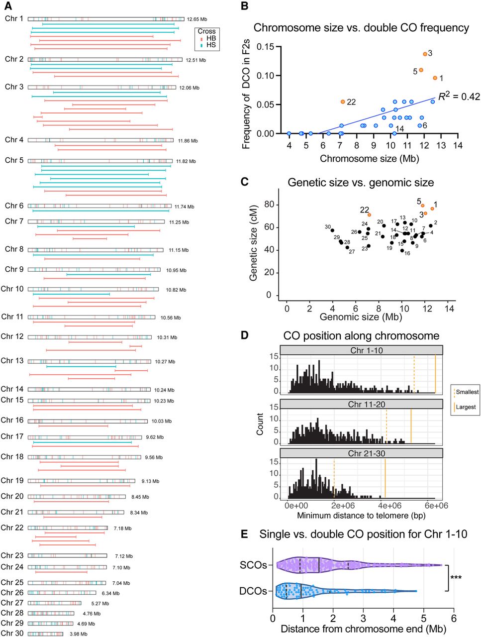
In addition to possible chromosome-specific biases in DCO formation, we also found that COs are not randomly distributed along the chromosome length in Plodia. For all chromosomes, we found that COs in our sequencing data are significantly skewed toward chromosome arms (the outer-most third of the chromosome), with this bias being most pronounced for larger chromosomes (Fig. 3D; Supplemental Fig. S7B,C; Supplemental Table S3). However, when we plotted CO position as a normalized distance from the nearest telomere for large, medium, or small chromosomes, we observed similar distributions regardless of chromosome size (Fig. 3D), in which COs are most likely to form ∼1–2.5 Mb (median = 1.5 Mb) from the telomere and not at a specific position on the chromosome (arm vs. center). This is similar to data from both plants and animals, including the roundworm Caenorhabditis elegans in which COs form ∼0.6–1 Mb from the chromosome ends (Saito and Colaiácovo 2017; Haenel et al. 2018; Castellani et al. 2024). When DCOs form on long chromosomes, these two COs are even more distal than SCOs on the same chromosomes, with DCOs forming only 0.5–2 Mb (median = 1 Mb) from the telomere (Fig. 3E), further supporting the presence of strong CO interference in Plodia.
COs are not enriched in gene bodies, GC-rich regions, or TEs
In C. elegans, the distal chromosome arms in which COs tend to form are more gene-poor compared with chromosome centers. However, in Plodia and most moths, genes are more uniformly distributed across chromosomes (Supplemental Fig. S9; Rosin et al. 2021; Hockens et al. 2024). Still, we wondered whether it is still possible for COs to be depleted from genes on the chromosome arms. Using Fisher's exact tests followed by multiple testing adjustments with our F2 sequencing data, we find that COs are, in general, mildly depleted from gene bodies (adjusted P-value = 0.007, odds ratio = 0.84). Of those COs that were found in genes, they are significantly more likely to be in introns than in exons (adjusted P-value = 2.11 × 10⁻⁷, odds ratio = 1.69), and COs are significantly depleted from promoters defined as transcript-level transcription start sites (TSSs) ±500 bp (adjusted P-value = 4.7 × 10⁻⁵, odds ratio = 0.6). Among COs that do fall within genes, the genes on chromosome arms are actually enriched for COs compared with those in the middle of the chromosome (adjusted P-value = 1.1 × 10⁻¹⁵, odds ratio = 1.89). Together, this means COs tend to be less common in genes throughout the genome, but they still occur in genes located on chromosome arms rather than being excluded from them.
Similarly, GC-rich chromatin has been associated with meiotic CO formation in both plants and animals and is often associated with open/active chromatin domains (Eyre-Walker 1993; Glémin et al. 2014; Rodgers-Melnick et al. 2015; Hinch et al. 2019). In Plodia, we find that GC content is relatively even across chromosomes apart from the AT-rich telomeric repeats (Supplemental Fig. S10; Okazaki et al. 1993; Vítková et al. 2005). We find no significant correlation between GC content and CO position (Pearson's correlations over 1 kb windows range from −0.01 to 0.01, depending on the chromosome).
Because COs are not enriched in gene bodies or GC-rich domains, we wondered if they might be enriched in TEs, which we showed above are also enriched in chromosome arms (Supplemental Fig. S4; Supplemental Data Set S1). To test this, we calculated the observed occurrence of COs in TEs and compared it to the expected occurrence by chance (Supplemental Data Set S3). Although some COs do fall within TEs and other repeats, we did not observe a significant enrichment of COs in TEs or any other repetitive sequences (adjusted P-value = 0.27, odds ratio = 1.09) (Supplemental Data Set S3; Supplemental File S1). Importantly, we also did not see a correlation between COs and variants in either strain, with Pearson's correlations over 1 kb windows being between –0.014 and 0.038 for Savannah-specific variants and −0.0047 and 0.035 for bFog-specific variants. Thus, COs are not enriched in TEs and are not significantly associated with genetic variants in either strain.
COs are more likely to occur in heterochromatic chromosome regions
Because we did not observe an enrichment of COs in TEs, genes, or GC-rich chromatin, we wondered what makes chromosome arms a more hospitable environment for CO formation in Plodia. To this end, we generated the first comprehensive chromatin landscape map for Plodia testes by performing CUT&RUN, ATAC-seq, and RNA-seq to map histone modifications, chromatin accessibility, and transcription, respectively (Fig. 4A; Supplemental Fig. S12). This was done in whole larval testes, in which a large fraction of cells are in meiotic prophase I (Supplemental Fig. S11A,B; Buenrostro et al. 2015; Skene and Henikoff 2017; Rosin et al. 2021).
COs occur in heterochromatic regions of the genome in Plodia. (A) Screenshot of select CUT&RUN and ATAC-seq tracks for a representative genomic locus on Chr 29. Each track represents merged views of two to four biological replicates. (B, left) Eight-state ChromHMM model emission values; darker blue indicates a higher likelihood of finding that mark in that state. (Right) Heat map showing enrichment for specific features (listed below) in each state; darker black indicates a higher likelihood of that feature being in that state. Columns have been divided by column-wise maximum. (C) Histogram showing the minimum distance of state designations (states 3, 7, and 8) from the end of a chromosome, in which the number of loci is binned using 30 kb windows. The genome was subdivided into three chromosome-sized groups, with Chr 1–10 (largest; 12.65–10.82 Mb) shown at the top, Chr 11–20 (10.56–8.45 Mb) shown in the middle, and Chr 21–30 (smallest; 8.34–3.98 Mb) shown at the bottom.
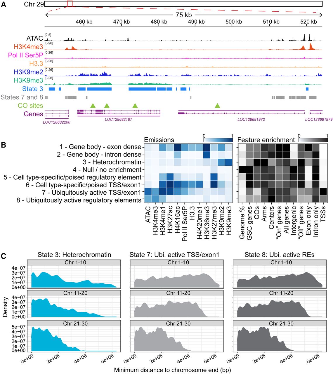
CUT&RUN was used to map the following histone modifications: H3K4me1, H3K4me3, H3K9me2, H3K9me3, H3K27me3, H3K36me3, H3K27ac, H4K16ac, H4K20me1, H3.3, and RNA polymerase II CTD ser5 phosphorylation (Pol II Ser5P) (Fig. 4A,B). Using these data, we then trained hidden Markov models with ChromHMM to segment the genome into different nonoverlapping chromatin states in larval testes and determine if COs are enriched within any specific state (Ernst and Kellis 2012). After manual inspection of models built with up to 15 states, we selected the eight-state model for its interpretability. Based on the histone marks associated with each state, as well as the enrichment of certain genomic features within the states, such as annotated gene introns/exons or TSSs, we classified each of the eight states as follows (Fig. 4B). State 8 was characterized by high emission probabilities for ATAC signal, H3K4me3, and H3K4me1, which are all marks of gene enhancers and promoters; thus, we classified state 8 as “ubiquitously active regulatory elements” (meaning active in all cell types in the testes). State 7 was enriched for ATAC signal, H3K4me3, and H3K4me1 in addition to Pol II Ser5P, H3K27ac, and H4K16ac (marks of active promoters and active transcription), and thus, we classified state 7 as “ubiquitously active TSS/exon 1.” State 6 was enriched for marks associated with active transcription, but not active promoters, and showed increased H3K27me3, a mark associated with spatial or temporal silencing. Thus, we classified state 6 as “cell-type-specific or poised TSS/exon 1.” State 5 showed enrichment for both H3K4me1 (active promoters) and H3K27me3 (silencing) and was therefore classified as “cell-type-specific or poised regulatory elements.” State 4 had no specific enrichment and was classified as “null” chromatin. State 3 was enriched for H3K9me2 and H3K9me3, marks of constitutive silencing and, as such, was classified as “heterochromatin.” Finally, states 1 and 2 are most enriched for H4K16ac and H3K36me3, marks of active transcription, and were classified as “gene body–exon dense” and “gene body–intron dense,” respectively, based on their location enrichment in the genome.
To validate these classifications, we looked at several genomic features to see which state(s) they most associated with. We found that most of the genome falls into the null/no enrichment state (Fig. 4B) in which no signal is detected. In agreement with states 5 and 6 being “cell-type-specific” or “poised” states, we found that germline stem cell (GSC) genes, which should only be expressed in a specific subset of cells in testes, are most enriched for states 5 and 6 (Fig. 4B). We confirmed that annotated intergenic regions of the genome are depleted from states 1 and 2 (“gene bodies”), and annotated TSSs are enriched in states 7 and 8 (Fig. 4B).
When we looked at the location of these states genome-wide, we found that only states 3 (“heterochromatin”), 7, and 8 (“ubiquitously active regulatory elements”) show biases in their genomic position. State 3 is more enriched within chromosome arms, and conversely, states 7 and 8 are more enriched toward chromosome centers, especially for big chromosomes (Fig. 4B,C; Supplemental Fig. S13). Correspondingly, we found that COs are most enriched within state 3 (darker gray box) and are largely depleted from states 7 and 8 (lightest gray boxes) (Fig. 4A,B; Supplemental Fig. S13). Together, these data suggest that although chromosome arms are not necessarily gene-poor based on the current annotations for the Plodia genome (Supplemental Fig. S9), they are indeed more heterochromatic than chromosome centers based on our ChromHMM analysis. These findings suggest that closed chromatin may be more permissive for CO formation in Plodia.
Altogether, the data presented here support a model in which the pantry moth P. interpunctella harbors robust CO assurance and interference with COs showing a general enrichment in heterochromatic regions of chromosome arms.
Discussion
CO designation and the impact of CO variation are notoriously difficult to study in humans and mammalian model systems, in which CO formation occurs in only a subset of cells in testes or in fetal ovaries and rearing hundreds of mice for CO mapping experiments is extremely cost prohibitive. Here, we employ the genetically tractable pantry moth, P. interpunctella, to investigate CO formation in a new model system with a large number of chromosomes using a high-throughput sequencing approach. We performed whole-genome sequencing to generate SNP maps for the Savannah and the bFog Plodia laboratory strains. Because these are not isogenic strains, we were able to capture a robust amount of “between strain” and “within strain” variants. Why so much genetic variation exists in Plodia is still unclear, but one possibility is that this is caused by population bottlenecks with small laboratory culturing. The amount of genetic variation in our strains contrasts with the notion that lepidopteran genomes are highly stable (Traut et al. 2023) and instead supports a model in which lepidopteran genomes rapidly evolve (Wright et al. 2024).
Consistent with previous studies in Lepidoptera, our sequencing-based approach showed that COs are present in male meiosis but absent during female meiosis in Plodia (Maeda 1939; Holm and Rasmussen 1980; Rasmussen and Holm 1982; Rasmussen 1986, 1987; Shipilina et al. 2022; Xiong et al. 2023). Most of these studies have suggested that SCOs are predominant in lepidopteran spermatogenesis (Kaback et al. 1992; Jiggins et al. 2005; Yasukochi et al. 2006), which is also true in our data set. However, we did observe DCO and NoCO events by both sequencing and DNA FISH. It is important to note that the relatively small sample size here (n = 73 individuals for sequencing and 668 round spermatids from two gonads quantified by FISH) could skew the percentages of rare events such as NoCOs and DCOs.
The observation of frequent SCOs and limited NoCOs and DCOs combined with our CoC analyses suggest strong CO assurance and interference in Plodia. The predicted level of CO assurance in Plodia based on the Weinstein tetrad analysis (in which only ∼5% of bivalents are predicted to lack COs) is lower than that reported for another holocentric species, C. elegans, in which essentially all bivalents receive a SCO. It is, instead, similar to other insects like Drosophila, in which chromosome arms fail to receive COs only ∼10% of the time (except for Chr 4, which lacks COs entirely and instead relies on an alternative segregation mechanism) (Comeron et al. 2012; Miller et al. 2016; Saito and Colaiácovo 2017; Hawley et al. 2025).
In Drosophila, although it is unusual for any of the three main chromosomes to entirely lack COs, it is possible. In NoCO situations, Drosophila use a back-up segregation system to ensure all chromosomes are segregated equally (for review, see Hughes et al. 2018). We believe that NoCO bivalents in Plodia may similarly be segregated via an alternative “back-up” mechanism. We previously showed in silk moths that the synaptonemal complex persists through metaphase I in spermatogenesis, possibly helping to keep the homologs linked when COs do not form, similar to the mechanism in achiasmatic female meiosis (Xiang et al. 2024; Benner et al. 2026). In agreement with lepidopteran insects having a back-up mechanism for homolog linkage, a recent study in Papilio butterflies found something similar to what we observed here in Plodia, in which NoCOs were observed along with SCOs and DCOs (Xiong et al. 2023). These studies, combined with our data from Plodia, suggest that CO assurance might be more of a challenge for moths than for flies, perhaps owing to the increased number or smaller size of chromosomes in lepidopteran systems. Still, the mechanisms regulating CO assurance in systems with large numbers of chromosomes are not well understood and should be the subject of future studies.
Another difference we observed in CO regulation between Plodia and other invertebrates is the levels of CO interference. For example, C. elegans have extremely robust CO interference, with DCOs almost never being observed (Yokoo et al. 2012). Our Weinstein tetrad analysis of the Plodia data, on the other hand, suggests that Plodia could have DCOs up to 50% of the time for some chromosomes. This would indicate that levels of CO interference are not directly correlated with chromosome size between different species, as Plodia chromosomes are much smaller than C. elegans chromosomes (only ∼4–13 Mb in Plodia compared with ∼14–20 Mb in C. elegans). In agreement with the idea that chromosome size and CO formation are not directly linked, we also did not see a significant correlation between chromosome size and CO number within the Plodia genome, both for our raw F2 CO numbers and the Weinstein tetrad estimates. Although our Weinstein tetrad estimates suggest that some Plodia chromosomes may harbor DCOs up to 50% of the time, other chromosomes of similar or even larger sizes are only predicted to get two COs 5%–10% of the time. A similar phenomenon was observed in Papilio, with chromosomes of similar sizes being differentially susceptible to DCOs (Xiong et al. 2023). At least in Plodia, this seems to be independent of the amount of heterochromatin or accessible chromatin per chromosome based on our ChromHMM analysis (Supplemental Fig. S14).
One possible explanation for the differences in CO interference not directly correlating with the chromosome size is the fact that CO interference is influenced by chromosome axis length at pachytene (Kleckner 2006; Wang et al. 2017). Perhaps axis length does not scale proportionally with chromosome genomic size in moths and butterflies. That is to say, Chr 1, 3, and 5 may form more DCOs than Chr 2, 4, or 6 owing to longer chromosome axis length on Chr 1, 3 and 5, independent of genomic size, but this possibility has yet to be explored. Another possibility is that pairing timing might differ between these chromosomes, with “earlier pairing” chromosomes perhaps being more likely to form multiple COs. Several factors can impact the timing of pairing, including gene density and nuclear position/organization before pairing (MacQueen and Villeneuve 2001; Marshall and Fung 2016; Hockens et al. 2024).
Importantly, previous and new (this study) FISH-based quantifications of bivalent structures at metaphase I in Plodia spermatogenesis support these Weinstein predictions of chromosome-specific DCO biases (Supplemental Fig. S8A–C; Hockens et al. 2024). For all chromosomes examined by FISH, we observe two distinct post-CO structures at metaphase I: rod-shaped bivalents with one arm linked between the homologs and the other arm facing the spindle pole, and ring-shaped bivalents with both arms linked and the center of the chromosome facing the spindle pole (Supplemental Fig. S8; Hockens et al. 2024). We believe that rod-shaped bivalents result from a single, distal CO, whereas ring-shaped bivalents form after two distal COs. Consistent with the Weinstein estimates, we find that some chromosomes are more likely to form ring-shaped bivalents (two COs) than others of a similar size (e.g., Chr 3 and 5 show more DCO ring-shaped bivalents by FISH and also in the Weinstein estimates based on our sequencing-based mapping of COs) (Supplemental Fig. S8B,C). Still, it is also possible that these variations in predicted DCO frequency are exaggerated based on the Weinstein tetrad analysis, and they may not be biologically significant.
Although CO assurance and interference seem to differ slightly between moths and other holocentric invertebrates like C. elegans, we did find some similarities in CO position between Plodia and C. elegans. Specifically, in C. elegans, COs are also enriched in the heterochromatic chromosome arms, as we observed in Plodia (Barnes et al. 1995; Rockman and Kruglyak 2009; Gerstein et al. 2010; Ikegami et al. 2010; Liu et al. 2011; Lascarez-Lagunas et al. 2023). This is distinct from the placement of COs in many other systems, in which COs tend to be enriched in more open, active chromatin domains. For example, in many mammals, DSB formation is PRDM9 dependent. PRDM9 is a zinc finger DNA binding protein that binds to specific DNA motifs in which it deposits active histone marks. Therefore, COs form in active chromatin regions in mammals with PRDM9 (Baudat et al. 2010; Myers et al. 2010; Parvanov et al. 2010; Powers et al. 2016; Paigen and Petkov 2018). In yeast or mammals lacking PRDM9, DSBs and COs are biased toward other open chromatin regions like gene promoters (Pan et al. 2011). Similarly, studies in Drosophila have suggested that COs tend to avoid heterochromatin during oogenesis (Mehrotra and McKim 2006; Adrian et al. 2016; Hughes et al. 2018). Thus, although chromatin architecture is known to influence the CO landscape across systems, why holocentric species like C. elegans and Plodia preferentially place COs in heterochromatin is still unclear. It could have something to do with the holocentric chromosome architecture, or COs might be enriched in heterochromatin by other/secondary factors in these systems.
In nearly all systems studied to date, COs are enriched toward chromosome ends and away from chromosome centers (Haenel et al. 2018). Could it be that regardless of chromatin environment at chromosome ends, COs will form a minimum distance from the end of chromosomes? There are many models suggesting why such a phenomenon might be true. For example, early chromosome pairing dynamics in meiotic prophase in most systems involves telomere anchoring to the nuclear envelope and telomere-led chromosome movements (Scherthan et al. 1996; Harper et al. 2004; Naranjo and Corredor 2008; Zickler and Kleckner 2016). Similarly, synaptonemal complex assembly and DSB formation have been shown to initiate at telomere-proximal loci in several systems (Croft and Jones 1989; Lukaszewski 1997; Bass et al. 2000; Anderson and Stack 2005; Brown et al. 2005; Viera et al. 2009; Higgins et al. 2014; Klutstein and Cooper 2014; Pratto et al. 2014; Xiang et al. 2014). Together, these telomeric “head starts” to pairing and synapsis could explain why CO repair might also be more likely near telomeres (Scherthan et al. 1996; Zickler and Kleckner 2016).
In summary, this study suggests an evolutionary conservation of the meiotic CO landscape between divergent holocentric species while at the same time revealing unique evolutionary signatures of the Plodia genome. How COs become restricted to chromosome arms in different holocentric systems is unknown, and the role that a “centromere effect” may have on CO formation in holocentric lineages is still unclear. One unique aspect of Plodia CO formation compared with other previously studied holocentric species is the large number of chromosomes in Plodia. There is generally a lack of information on mechanisms of CO assurance in species with large numbers of chromosomes, like moths and mammals. Thus, future studies interrogating mechanisms of CO assurance and designation in Plodia will be critical for progress in understanding CO assurance and for addressing the impact that rapid genome evolution can have on the CO landscape.
The strong CO assurance and interference observed here establish Plodia as a powerful model for more directed molecular studies on CO mechanisms in systems with large numbers of chromosomes in the future. Finally, uncovering CO distributions and the genetic architecture of CO variation in a new system, as we have done here, will provide key information for researchers studying the links between genetic diversity, fertility, and disease.
Methods
Plodia strains
Two nonisogenic P. interpunctella strains, Savannah (assembly data at NCBI Genomes database [https://www.ncbi.nlm.nih.gov/home/genomes/] under accession number GCF_027563975.2) and bFog (sequence data at NCBI Genomes BioProject database [https://www.ncbi.nlm.nih.gov/bioproject/] under accession number PRJNA610057), were obtained from the USDA Agricultural Research Services (Savannah, Georgia, isolate, inbred since the 1960s) and The George Washington University (Dundee-Florida hybrid, inbred since 2020), respectively. Both strains were maintained on modified Plodia artificial diet (44% w/v coarse wheat bran, 5% Brewer's yeast flakes, 9% d-glucose, 30% glycerol, 3% canola oil, and 10% water) with 8 h light/16 h dark photoperiod and 60%–80% controlled humidity at 28°C. These strains were used for crosses to generate F1 and F2 hybrids.
Crosses
Plodia WT Savannah and bFog strains were synchronized as pupae in corrugated cardboard “hotels” and sorted by sex. Virgin adults between 1 and 3 days after eclosion were then mated in a 1.25 oz plastic souffle cup (Solo) containing a pinch of diet (∼0.2g) and ∼1 cm2 of Kimwipe to generate heterozygous F1 hybrids. These crosses were performed in both directions: (1) WT Savannah males crossed to WT bFog females and (2) WT bFog males crossed to WT Savannah females. To analyze the heterozygous loci resulting from COs generated in the F1 male testes, the F1 hybrid males were then backcrossed to WT Savannah female or WT bFog females to produce F2 offspring for downstream sequencing and CO analyses, labeled as “HS” and “HB,” respectively. To avoid capturing additional COs from F2 testes in our sequencing data, all F2s that were sequenced were either females or males with testes removed. All F1 and F2 crosses were reared at room temperature (∼25°C) with ambient humidity (20%–40%).
PacBio and Illumina whole-genome sequencing
Detailed methods for whole-genome sequencing and analyses can be found in the Supplemental Methods. Briefly, PacBio long-read whole-genome sequencing of both Savannah and bFog strains (three individuals per strain) was performed using DNA from three fifth instar Savannah female larvae and three fifth instar bFog female larvae. PacBio libraries were generated using SMRTbell prep kit 3.0 with barcoded adapters; library QC was performed; and libraries were sequenced on a PacBio Sequel IIe system. PacBio circular consensus sequence (CCS) reads were converted to FASTQ format, and reads were assembled into contigs. Assembled contigs were checked for quality and aligned to the Savannah reference genome for visual inspection. QC metrics for the PacBio draft contig assemblies of Savannah and bFog strains can be found in Supplemental Table S4. The unassembled PacBio data were analyzed for both short and structural variants as described in the Supplemental Methods.
Illumina whole-genome sequencing was performed on three WT bFog and three WT Savannah female larvae, as well as 10 F1 hybrid females and 83 F2 hybrids (73 females, 10 males with gonads removed), for haplotype mapping and for looking for COs. Briefly, fifth instar larvae were thoroughly pulverized in a tube on dry ice using a pestle. Genomic DNA was extracted and used for generating Illumina libraries using DNA prep kit (Illumina) according to the manufacturer's protocol. Library QC was performed, and libraries were sequenced on an Illumina NovaSeq 6000 with SP200 flow cell (100 bp paired-end). Illumina data were analyzed for short variants as described below.
ATAC-seq, RNA-seq, and CUT&RUN library generation and sequencing
Detailed methods for library preparation and sequencing can be found in the Supplemental Methods. Briefly, testes for ATAC-seq (Buenrostro et al. 2015) were dissected from fifth instar WT bFog male larvae, homogenized, strained, and cells were counted. A total of ∼100,000 cells per replicate were used for tagmentation using the Active Motif ATAC-seq Kit (catalog 53150). Libraries were sequenced on an Illumina NovaSeq 6000 with SP100 flow cell (50 bp paired-end). Raw data can be accessed from NCBI (see Data access).
For RNA-seq, testes were dissected from fifth instar WT bFog larvae in ice-cold PBS. Total RNA was isolated using the RNeasy plus kit (Qiagen). Samples were purified and barcoded using TruSeq stranded mRNA library prep kit (Illumina). All libraries were pooled and sequenced on an Illumina NovaSeq 6000 with SP200 flow cell (100 bp paired-end).
For CUT&RUN (Skene and Henikoff 2017), cells were isolated from fifth instar WT bFog larval testes and pulverized with a pestle in a 1.5 mL tube. About 500,000 cells were harvested per reaction. CUT&RUN was performed using the CUTANA ChIC/CUT&RUN kit (EpiCypher) following the manufacturer's protocol. CUT&RUN libraries were generated using NEBNext Ultra II DNA library prep kit for Illumina (New England Biolabs). Libraries were sequenced on an Illumina NovaSeq 6000 with SP100 flow cell (50 bp paired-end). A complete list of antibodies used for CUT&RUN can be found in Supplemental Table S5. Detailed ATAC-seq, RNA-seq, and CUT&RUN analyses methods can be found in the Supplemental Methods.
Downstream analysis of variants from whole-genome sequencing data
Downstream analysis of the Illumina short variants involved generating coverage tracks and colored variant tracks for F2 hybrids. First, Illumina short variants, PacBio short variants, and PacBio structural variants (“union”) were combined for both WT Savannah and WT bFog individuals to define the largest possible set of variants (“complete”) observed in each strain. Next, for each F2 “HS” hybrid, all Savannah “complete” variants were removed, and only variants that also appeared in the bFog “complete” variant set were kept. This translates to the set operation: (F2–“Savannah complete”) ∩ “bFog complete.” For each F2 “HB” hybrid, the reciprocal operation was performed: (F2–“bFog complete”) ∩ “Savannah complete.” Finally, the remaining variants were binned in 200 bp windows across the genome to generate coverage tracks. Note that WT variants were not filtered by any criteria to cast the widest possible net of potential variant sites, whereas the F2 variants were only subjected to a minimal depth filter (minimum depth ≥ 10 reads).
Coverage tracks for F2 “HB” hybrids were very sparse, owing to the large number of differences from the Savannah reference genome across most chromosomes. To address this, an alternate visualization was generated as follows: Genotypes of variants observed in F2 “HB” hybrids were compared directly with WT Savannah and WT bFog parents and classified into four groups: “Savannah-like,” “bFog-like,” “het,” or “unknown.” An F2 variant was classified as “unknown” if variants in WT parents were (1) multiallelic, (2) identical to the F2 variant (uninformative sites), or (3) absent or unknown (genotype “./.”) in WT parents. If the F2 variant exactly matched the Savannah or bFog parent, it was classified as “Savannah-like” or “bFog-like,” respectively. Finally, any remaining variant with a heterozygous genotype was classified as “het.” For visualization purposes, adjacent identical calls within 200 bp were merged together.
Any loci in which a single individual differed from the other individuals in the strain were classified as “intrastrain” variants. Loci that were nonvariant within each strain (all three individuals had the same allele) but differed between strains were classified as “interstrain” variants and were further used for haplotype generation and Oligopaints design.
The resolution for mapping COs from our data was calculated using the following procedure. First, all F2 variants classified as “unknown” were removed; for “HS” and “HFS” backcrosses, regions of intrastrain variation were removed. Next, the distance between adjacent calls for each chromosome was calculated, and the median was computed. Finally, the median distances were aggregated across all individuals to obtain a population estimate. This procedure yielded the following resolution estimates for each cross: “HS,” 53–72 bp; “HB,” 54–76 bp; and “HFS,” 57–62 bp. Skewness of variant distributions near chromosome ends within chromosome length bins for Savannah and bFog was calculated using the “skewness” function from the “e1071” R package (R Core Team 2024).
TE and satellite repeat identification and analysis
De novo identification of TEs and other repeats in the P. interpunctella genome was performed using the RepeatModeler v2.0.1 tool (with -pa 8 -LTRStruct settings, and using rmblast 2.10.0+ search engine) (Flynn et al. 2020) independently on the reference assembly (ilPloInte3.2, GCF_027563975.2) and on each of the two strain-specific PacBio contig assemblies produced in this study (WT bFog and WT Savannah). The repeat library resulting from the modeling based on the reference assembly was used to annotate TEs and other repeats in the reference genome using RepeatMasker v4.1.9 (with sensitive mode and rmblastn version 2.14.1+) (Smit et al. 2013). This annotation was used for all downstream analysis of repeats, with the only exception of satellite sequences. Graphical representation of TE abundance by class was performed using the R package ggplot2 (Wickham 2016).
Satellite consensus sequences were identified only in the repeat libraries obtained from the repeat modeling on strain-specific PacBio contig assemblies. Satellite consensus sequences were subsequently annotated in the reference assembly using either the bFog or the Savannah repeat library.
Alignment of the bFog and Savannah satellite consensus sequences was performed using Clustal Omega (Sievers et al. 2011) with default settings. The intersect command in BEDTools (-wao option) (Quinlan and Hall 2010) was used to identify overlap of satellite repeats annotated in the reference assembly using the consensus sequences obtained with either the bFog or Savannah repeat library. Venn diagram was plotted using the R package eulerr v7.0.2 (https://github.com/jolars/eulerr).
To compare TE and CO density on chromosome arms (first and last third of each chromosome) versus center (middle third of each chromosome), an analysis was performed similarly to that described previously (Teterina et al. 2020). Briefly, density of TEs and COs over the reference genome was calculated using the BEDTools coverage command (100 kb windows). The Cohen's d effect size test was performed to measure positional effect of TEs and COs distribution on chromosome arms versus center using the R package lsr v0.5.2 (https://learningstatisticswithr.com/), and statistical differences were calculated using the Wilcoxon rank-sum test in base R.
To test the enrichment of COs, bFog variants, and Savannah variants over TEs, a permutation test using 1000 permutations was performed for each TE class using the overlapPermTest function of the regioneR package with default settings (Gel et al. 2016). Ideogram plots were generated using the karyoploteR package (Gel and Serra 2017).
CO quantification and Weinstein tetrad analysis
CO positions were manually determined using coverage tracks (as shown in Fig. 2B; Supplemental Fig. S5B–E) or variant tracks (Supplemental Fig. S6A,B). Coverage tracks were used for WT Savannah backcrosses (HS) and variant tracks were used for WT bFog backcrosses (HB). To determine the approximate CO site(s) on each chromosome for each F2 individual, changes in heterozygosity status were determined to the closest base pair position between identifiable strain-specific variants. Skewness of CO distributions in chromosome length bins was calculated using the function “skewness” from the “moments” R package (R Core Team 2024). Coverage tracks and variant tracks were viewed in Integrative Genomics Viewer (IGV) (Thorvaldsdóttir et al. 2013). Chromosomes were examined on the whole-chromosome scale for changes in variant or heterozygosity patterns. For coverage tracks, CO site was determined by zooming into the base pair position at which bFog variants become present/absent on the chromosomes. For variant tracks, CO site was determined by zooming into the base pair position at which heterozygous genotypes become present/absent on the chromosomes. Three to five genomes from each cross were also analyzed by a second scorer, with identical results. Weinstein tetrad analysis was performed as previously described, using a public-facing web app (Hawley et al. 2025).
ChromHMM analysis
Detailed methods for ChromHMM analysis can be found in the Supplemental Methods. Briefly, CUT&RUN BAM files were merged with SAMtools merge (v1.22.1) (Danecek et al. 2021) to BED with BEDTools bamtobed (v2.3.1) (Quinlan and Hall 2010) and binarized with ChromHMM BinarizeBed (v1.27) (Ernst and Kellis 2017) using the default bin size. Models were trained using these binarized BED files as input to ChromHMM LearnModel. The enrichment within each state and the various enrichment tracks (for description, see Supplemental Methods) were evaluated with ChromHMM OverlapEnrichment. Details on enrichment track generation can be found in the Supplemental Methods.
CO interference calculations
CO interference was calculated based on previously published methods (Chuang and Smith 2023). A detailed version of our methodology can be found in the Supplemental Methods. Data for Drosophila were analyzed in the same fashion, and CO events were derived from published data (Miller et al. 2016).
Oligopaints’ design and synthesis
For the HOPs design, a slightly modified version of previously published pipelines was used (Beliveau et al. 2015; AlHaj Abed et al. 2019). Detailed methods for Oligopaints’ design and synthesis can be found in Supplemental Methods.
Oligo pools were ordered from Twist Biosciences and paints were synthesized in-house as previously described, using the T7 method (Rosin et al. 2018; Nguyen and Joyce 2019).
Oligopaints FISH and quantification
Testes squashes and downstream Oligopaints FISH were performed as previously described (Rosin et al. 2021) using testes from fifth instar Plodia larvae. For detailed methods, see Supplemental Methods. COs based on HOPs probes on round spermatids were quantified manually. Data were collected from two testes (two replicates), totaling 668 nuclei.
Immunofluorescence and quantification
Plodia HEI10 was identified by BLAST search using the Bombyx mori HEI10 protein as bait (Benner et al. 2026). A HEI10 peptide (CGSELRDKFDVIQADLKPSETFKS) was synthesized, purified, and used for monospecific polyclonal antibody generation via Pacific Immunology. Plodia SYCP3 antibody was previously published by our laboratory (Burns et al. 2026).
Immunofluorescence with HEI10 and SYCP3 antibodies was performed on spermatocyte spreads from WT bFog males, the protocol for which was adapted from previously published protocols (Xiang et al. 2023; Horan 2025). For the detailed protocol, see Supplemental Methods.
Quantified data were collected from two biological replicates, totaling about 50 cells. Foci quantification was performed on maximum projections in ImageJ using auto thresholding and the “analyze particles” function.
Imaging
Oligopaints on testes squashes were imaged using a Leica DMi8 widefield inverted fluorescence microscope equipped with APO 63X/1.40 CS2 oil objective (Leica), K8 CMOS monochrome camera, LED8 light source, and DAPI/FITC/CY3/CY5/CY7 filter cubes. Images were processed using Huygens Professional express deconvolution, and tiffs were created in ImageJ.
For DAPI stain on whole-mount testes and spermatocyte spread immunofluorescence, images were acquired on a Leica Stellaris 8 resonant scanning confocal with four HyD S detectors and one HyD X SP detector, as well as the SuperZ Galvo stage. Images were postprocessed with Leica Lightning superresolution software or Huygens Professional express deconvolution, and tiffs were generated in ImageJ.
Data access
The RNA-seq and ATAC-seq data generated in this study have been submitted to the NCBI BioProject database (https://www.ncbi.nlm.nih.gov/bioproject/) under accession number PRJNA1278932. PacBio and Illumina whole-genome sequencing data generated in this study are available under accession number PRJNA1397214. CUT&RUN data generated in this study are available under accession number PRJNA1403002. The analysis code used in this study is available at GitHub (https://github.com/NICHD-BSPC/lee-2026) and as Supplemental Code.
Competing interest statement
The authors declare no competing interests.
Acknowledgments
We acknowledge the late Dr. Scott Hawley for his input and suggestions on the early stages of this project, and Dr. Andre Marques for discussions at the early stages of this project. We thank Dr. Christa Heryanto for assistance with Plodia rearing and crosses. This work utilized the computational resources of the NIH HPC Biowulf cluster (https://hpc.nih.gov). We also thank Dr. Takashi Akera, Dr. Alex Kelly, and their laboratories for helpful discussions. Finally, we thank Dr. Stacie Hughes and Dr. Michael Lichten for suggestions and critical reading of the manuscript. This research was supported by the Intramural Research Program of the National Institutes of Health (NIH). The contributions of the NIH author(s) are considered works of the U.S. government. The findings and conclusions presented in this paper are those of the authors and do not necessarily reflect the views of the NIH or the U.S. Department of Health and Human Services. Specifically, this work was funded by the Eunice Kennedy Shriver National Institute of Child Health and Human Development, NIH (ZIAHD009019 to L.F.R. and ZICHD008986 to R.K.D.; https://www.nichd.nih.gov/about/org/dir). The funders had no role in study design, data collection and analysis, decision to publish, or preparation of the manuscript.
Author contributions: L.S.L. was responsible for conceptualization, experimentation and methodology, data analysis, writing, and editing. A.M. was responsible for computation, code writing and optimization, data analysis, writing, and editing. L.B. was responsible for experimentation and methodology, computation, data analysis, and writing. M.B. was responsible for computation, data analysis, and writing. L.M.R. was responsible for computation and data analysis. R.K.R. was responsible for experimentation. E.S. was responsible for computation and Oligopaints design. R.K.D. was responsible for bioinformatic conceptualization, code writing and optimization, data analysis, writing, editing, and supervision. L.F.R. was responsible for conceptualization, Oligopaints design, data analysis, writing, editing, and supervision.
Footnotes
[1] Supplementary material [Supplemental material is available for this article.]
[2] Article published online before print. Article, supplemental material, and publication date are at https://www.genome.org/cgi/doi/10.1101/gr.281913.126.
[3] Freely available online through the Genome Research Open Access option.
References
- ↵Adrian AB, Corchado JC, Comeron JM. 2016. Predictive models of recombination rate variation across the Drosophila melanogaster genome. Genome Biol Evol 8: 2597–2612. 10.1093/gbe/evw181
- ↵AlHaj Abed J, Erceg J, Goloborodko A, Nguyen SC, McCole RB, Saylor W, Fudenberg G, Lajoie BR, Dekker J, Mirny LA, 2019. Highly structured homolog pairing reflects functional organization of the Drosophila genome. Nat Commun 10: 4485. 10.1038/s41467-019-12208-3
- ↵Anderson LK, Stack SM. 2005. Recombination nodules in plants. Cytogenet Genome Res 109: 198–204. 10.1159/000082400
- ↵Arter M, Keeney S. 2024. Divergence and conservation of the meiotic recombination machinery. Nat Rev Genet 25: 309–325. 10.1038/s41576-023-00669-8
- ↵Baril T, Hayward A. 2022. Migrators within migrators: exploring transposable element dynamics in the monarch butterfly, Danaus plexippus. Mob DNA 13: 5. 10.1186/s13100-022-00263-5
- ↵Barnes TM, Kohara Y, Coulson A, Hekimi S. 1995. Meiotic recombination, noncoding DNA and genomic organization in Caenorhabditis elegans. Genetics 141: 159–179. 10.1093/genetics/141.1.159
- ↵Bass HW, Riera-Lizarazu O, Ananiev EV, Bordoli SJ, Rines HW, Phillips RL, Sedat JW, Agard DA, Cande WZ. 2000. Evidence for the coincident initiation of homolog pairing and synapsis during the telomere-clustering (bouquet) stage of meiotic prophase. J Cell Sci 113: 1033–1042. 10.1242/jcs.113.6.1033
- ↵Baudat F, Buard J, Grey C, Fledel-Alon A, Ober C, Przeworski M, Coop G, de Massy B. 2010. PRDM9 is a major determinant of meiotic recombination hotspots in humans and mice. Science 327: 836–840. 10.1126/science.1183439
- ↵Beliveau BJ, Boettiger AN, Avendaño MS, Jungmann R, McCole RB, Joyce EF, Kim-Kiselak C, Bantignies F, Fonseka CY, Erceg J, 2015. Single-molecule super-resolution imaging of chromosomes and in situ haplotype visualization using Oligopaint FISH probes. Nat Commun 6: 7147. 10.1038/ncomms8147
- ↵Benner L, Richmond M, Xiang Y, Lee L, Hockens CB, Li T, Yu Z, Tsuchiya D, Huang S, Tromer EC, 2026. Programmed meiotic errors facilitate dichotomous sperm production in the silkworm, Bombyx mori. Proc Natl Acad Sci 123: e2520991123. 10.1073/pnas.2520991123
- ↵Bolcun-Filas E, Handel MA. 2018. Meiosis: the chromosomal foundation of reproduction. Biol Reprod 99: 112–126. 10.1093/biolre/ioy021
- ↵Bomblies K, Higgins JD, Yant L. 2015. Meiosis evolves: adaptation to external and internal environments. New Phytol 208: 306–323. 10.1111/nph.13499
- ↵Brekke C, Johnston SE, Knutsen TM, Berg P. 2023. Genetic architecture of individual meiotic crossover rate and distribution in Atlantic Salmon. Sci Rep 13: 20481. 10.1038/s41598-023-47208-3
- ↵Brown PW, Judis L, Chan ER, Schwartz S, Seftel A, Thomas A, Hassold TJ. 2005. Meiotic synapsis proceeds from a limited number of subtelomeric sites in the human male. Am J Hum Genet 77: 556–566. 10.1086/468188
- ↵Buenrostro J, Wu B, Chang H, Greenleaf W. 2015. ATAC-seq: a method for assaying chromatin accessibility genome-wide. Curr Protoc Mol Biol 109: 21.29.1–21.29.9. 10.1002/0471142727.mb2129s109
- ↵Burns EE, Amoiroglou A, Fagerstrom CJ, Ryniawec JM, Lee L, Runyan RK, Rosin LF, Rogers GC, Rusan NM. 2026. Visualizing Drosophila centrioles by expansion microscopy. J Cell Sci 139: jcs264338. 10.1242/jcs.264338
- ↵Castellani M, Zhang M, Thangavel G, Mata-Sucre Y, Lux T, Campoy JA, Marek M, Huettel B, Sun H, Mayer KFX, 2024. Meiotic recombination dynamics in plants with repeat-based holocentromeres shed light on the primary drivers of crossover patterning. Nat Plants 10: 423–438. 10.1038/s41477-024-01625-y
- ↵Chuang Y-C, Smith GR. 2023. Meiotic crossover interference: methods of analysis and mechanisms of action. Curr Top Dev Biol 151: 217–244. 10.1016/bs.ctdb.2022.04.006
- ↵Comeron JM, Ratnappan R, Bailin S. 2012. The many landscapes of recombination in Drosophila melanogaster. PLoS Genet 8: e1002905. 10.1371/journal.pgen.1002905
- ↵Croft JA, Jones GH. 1989. Meiosis in Mesostoma ehrenbergii ehrenbergii. IV. Recombination nodules in spermatocytes and a test of the correspondence of late recombination nodules and chiasmata. Genetics 121: 255–262. 10.1093/genetics/121.2.255
- ↵Danecek P, Bonfield JK, Liddle J, Marshall J, Ohan V, Pollard MO, Whitwham A, Keane T, McCarthy SA, Davies RM, 2021. Twelve years of SAMtools and BCFtools. GigaScience 10: giab008. 10.1093/gigascience/giab008
- ↵Dapper AL, Payseur BA. 2019. Molecular evolution of the meiotic recombination pathway in mammals. Evolution 73: 2368–2389. 10.1111/evo.13850
- ↵Darlington CD, Dark SOS. 1932. The origin and behaviour of chiasmata, II: Senobothrus parallelus. Cytologia (Tokyo) 3: 169–185. 10.1508/cytologia.3.169
- ↵Davis L, Smith GR. 2003. Nonrandom homolog segregation at meiosis I in Schizosaccharomyces pombe mutants lacking recombination. Genetics 163: 857–874. 10.1093/genetics/163.3.857
- ↵de Massy B. 2013. Initiation of meiotic recombination: how and where? Conservation and specificities among eukaryotes. Annu Rev Genet 47: 563–599. 10.1146/annurev-genet-110711-155423
- ↵Ernst J, Kellis M. 2012. ChromHMM: automating chromatin-state discovery and characterization. Nat Methods 9: 215–216. 10.1038/nmeth.1906
- ↵Ernst J, Kellis M. 2017. Chromatin-state discovery and genome annotation with ChromHMM. Nat Protoc 12: 2478–2492. 10.1038/nprot.2017.124
- ↵Eyre-Walker A. 1993. Recombination and mammalian genome evolution. Proc Biol Sci 252: 237–243. 10.1098/rspb.1993.0071
- ↵Finnegan DJ. 1989. Eukaryotic transposable elements and genome evolution. Trends Genet 5: 103–107. 10.1016/0168-9525(89)90039-5
- ↵Flynn JM, Hubley R, Goubert C, Rosen J, Clark AG, Feschotte C, Smit AF. 2020. Repeatmodeler2 for automated genomic discovery of transposable element families. Proc Natl Acad Sci 117: 9451–9457. 10.1073/pnas.1921046117
- ↵Foss E, Lande R, Stahl FW, Steinberg CM. 1993. Chiasma interference as a function of genetic distance. Genetics 133: 681–691. 10.1093/genetics/133.3.681
- ↵Gbadegesin MA. 2012. Transposable elements in the genomes: parasites, junks or drivers of evolution? Afr J Med Med Sci 41 Suppl: 13–25.
- ↵Gel B, Serra E. 2017. karyoploteR: an R/Bioconductor package to plot customizable genomes displaying arbitrary data. Bioinformatics 33: 3088–3090. 10.1093/bioinformatics/btx346
- ↵Gel B, Díez-Villanueva A, Serra E, Buschbeck M, Peinado MA, Malinverni R. 2016. regioneR: an R/Bioconductor package for the association analysis of genomic regions based on permutation tests. Bioinformatics 32: 289–291. 10.1093/bioinformatics/btv562
- ↵Gerstein MB, Lu ZJ, Van Nostrand EL, Cheng C, Arshinoff BI, Liu T, Yip KY, Robilotto R, Rechtsteiner A, Ikegami K, 2010. Integrative analysis of the Caenorhabditis elegans genome by the modENCODE project. Science 330: 1775–1787. 10.1126/science.1196914
- ↵Gerton JL, Hawley RS. 2005. Homologous chromosome interactions in meiosis: diversity amidst conservation. Nat Rev Genet 6: 477–487. 10.1038/nrg1614
- ↵Glémin S, Clément Y, David J, Ressayre A. 2014. GC content evolution in coding regions of angiosperm genomes: a unifying hypothesis. Trends Genet 30: 263–270. 10.1016/j.tig.2014.05.002
- ↵Gray S, Cohen PE. 2016. Control of meiotic crossovers: from double-strand break formation to designation. Annu Rev Genet 50: 175–210. 10.1146/annurev-genet-120215-035111
- ↵Haenel Q, Laurentino TG, Roesti M, Berner D. 2018. Meta-analysis of chromosome-scale crossover rate variation in eukaryotes and its significance to evolutionary genomics. Mol Ecol 27: 2477–2497. 10.1111/mec.14699
- ↵Harper L, Golubovskaya I, Cande WZ. 2004. A bouquet of chromosomes. J Cell Sci 117: 4025–4032. 10.1242/jcs.01363
- ↵Hawley RS, Price A, Li H, Jagannathan M, Staber C, Hughes SE, Williams S, Perera A, Egidy RR, Lawlor A, 2025. Patterns of crossover distribution in Drosophila mauritiana necessitate a re-thinking of the centromere effect on crossing over. Genetics 230: iyaf039. 10.1093/genetics/iyaf039
- ↵Heryanto C, Hanly JJ, Mazo-Vargas A, Tendolkar A, Martin A. 2022. Mapping and CRISPR homology-directed repair of a recessive white eye mutation in Plodia moths. iScience 25: 103885. 10.1016/j.isci.2022.103885
- ↵Higgins JD, Osman K, Jones GH, Franklin FCH. 2014. Factors underlying restricted crossover localization in barley meiosis. Annu Rev Genet 48: 29–47. 10.1146/annurev-genet-120213-092509
- ↵Hinch AG, Zhang G, Becker PW, Moralli D, Hinch R, Davies B, Bowden R, Donnelly P. 2019. Factors influencing meiotic recombination revealed by whole-genome sequencing of single sperm. Science 363: eaau8861. 10.1126/science.aau8861
- ↵Hockens C, Lorenzi H, Wang TT, Lei EP, Rosin LF. 2024. Chromosome segregation during spermatogenesis occurs through a unique center-kinetic mechanism in holocentric moth species. PLoS Genet 20: e1011329. 10.1371/journal.pgen.1011329
- ↵Holm PB, Rasmussen SW. 1980. Chromosome pairing, recombination nodules and chiasma formation in diploid Bombyx males. Carlsberg Res Commun 45: 483–548. 10.1007/BF02932921
- ↵Horan TSA. 2025. Preparation of meiotic chromosome spreads from mouse oocytes for assessment of synapsis and recombination. J Vis Exp (221). 10.3791/68749
- ↵Hughes SE, Miller DE, Miller AL, Hawley RS. 2018. Female meiosis: synapsis, recombination, and segregation in Drosophila melanogaster. Genetics 208: 875–908. 10.1534/genetics.117.300081
- ↵Ikegami K, Egelhofer TA, Strome S, Lieb JD. 2010. Caenorhabditis elegans chromosome arms are anchored to the nuclear membrane via discontinuous association with LEM-2. Genome Biol 11: R120. 10.1186/gb-2010-11-12-r120
- ↵Jiggins CD, Mavarez J, Beltrán M, McMillan WO, Johnston JS, Bermingham E. 2005. A genetic linkage map of the mimetic butterfly Heliconius melpomene. Genetics 171: 557–570. 10.1534/genetics.104.034686
- ↵Kaback DB, Guacci V, Barber D, Mahon JW. 1992. Chromosome size-dependent control of meiotic recombination. Science 256: 228–232. 10.1126/science.1566070
- ↵Keeney S, Lange J, Mohibullah N. 2014. Self-organization of meiotic recombination initiation: general principles and molecular pathways. Annu Rev Genet 48: 187–214. 10.1146/annurev-genet-120213-092304
- ↵Kleckner N. 2006. Chiasma formation: chromatin/axis interplay and the role(s) of the synaptonemal complex. Chromosoma 115: 175–194. 10.1007/s00412-006-0055-7
- ↵Klutstein M, Cooper JP. 2014. The chromosomal courtship dance-homolog pairing in early meiosis. Curr Opin Cell Biol 26: 123–131. 10.1016/j.ceb.2013.12.004
- ↵Kong A, Thorleifsson G, Frigge ML, Masson G, Gudbjartsson DF, Villemoes R, Magnusdottir E, Olafsdottir SB, Thorsteinsdottir U, Stefansson K. 2014. Common and low-frequency variants associated with genome-wide recombination rate. Nat Genet 46: 11–16. 10.1038/ng.2833
- ↵Kumar R, Bourbon H-M, de Massy B. 2010. Functional conservation of Mei4 for meiotic DNA double-strand break formation from yeasts to mice. Genes Dev 24: 1266–1280. 10.1101/gad.571710
- ↵Lascarez-Lagunas LI, Martinez-Garcia M, Nadarajan S, Diaz-Pacheco BN, Berson E, Colaiácovo MP. 2023. Chromatin landscape, DSB levels, and cKU-70/80 contribute to patterning of meiotic DSB processing along chromosomes in C. elegans. PLoS Genet 19: e1010627. 10.1371/journal.pgen.1010627
- ↵Lawlor MA, Ellison CE. 2023. Evolutionary dynamics between transposable elements and their host genomes: mechanisms of suppression and escape. Curr Opin Genet Dev 82: 102092. 10.1016/j.gde.2023.102092
- ↵Lenormand T, Dutheil J. 2005. Recombination difference between sexes: a role for haploid selection. PLoS Biol 3: e63. 10.1371/journal.pbio.0030063
- ↵Liu T, Rechtsteiner A, Egelhofer TA, Vielle A, Latorre I, Cheung M-S, Ercan S, Ikegami K, Jensen M, Kolasinska-Zwierz P, 2011. Broad chromosomal domains of histone modification patterns in C. elegans. Genome Res 21: 227–236. 10.1101/gr.115519.110
- ↵Lukaszewski AJ. 1997. The development and meiotic behavior of asymmetrical isochromosomes in wheat. Genetics 145: 1155–1160. 10.1093/genetics/145.4.1155
- ↵Lum PTM, Flaherty BR. 1970. Regulating oviposition by Plodia interpunctella1 in the laboratory by light and dark conditions. J Econ Entomol 63: 236–239. 10.1093/jee/63.1.236
- ↵MacQueen AJ, Villeneuve AM. 2001. Nuclear reorganization and homologous chromosome pairing during meiotic prophase require C. elegans chk-2. Genes Dev 15: 1674–1687. 10.1101/gad.902601
- ↵Maeda T. 1939. Chiasma studies in the silkworm, Bombyx mori L. Japanese J Genet 15: 118–127. 10.1266/jjg.15.118
- ↵Marshall WF, Fung JC. 2016. Modeling meiotic chromosome pairing: nuclear envelope attachment, telomere-led active random motion, and anomalous diffusion. Phys Biol 13: 026003. 10.1088/1478-3975/13/2/026003
- ↵Martin RH. 2006. Meiotic chromosome abnormalities in human spermatogenesis. Reprod Toxicol 22: 142–147. 10.1016/j.reprotox.2006.03.013
- ↵Mehrotra S, McKim KS. 2006. Temporal analysis of meiotic DNA double-strand break formation and repair in Drosophila females. PLoS Genet 2: e200. 10.1371/journal.pgen.0020200
- ↵Miller DE, Smith CB, Kazemi NY, Cockrell AJ, Arvanitakis AV, Blumenstiel JP, Jaspersen SL, Hawley RS. 2016. Whole-genome analysis of individual meiotic events in Drosophila melanogaster reveals that noncrossover gene conversions are insensitive to interference and the centromere effect. Genetics 203: 159–171. 10.1534/genetics.115.186486
- ↵Muller HJ. 1916. The mechanism of crossing-over. Am Nat 50: 193–221. 10.1086/279534
- ↵Myers S, Bowden R, Tumian A, Bontrop RE, Freeman C, MacFie TS, McVean G, Donnelly P. 2010. Drive against hotspot motifs in primates implicates the PRDM9 gene in meiotic recombination. Science 327: 876–879. 10.1126/science.1182363
- ↵Nambiar M, Chuang Y-C, Smith GR. 2019. Distributing meiotic crossovers for optimal fertility and evolution. DNA Repair (Amst) 81: 102648. 10.1016/j.dnarep.2019.102648
- ↵Naranjo T, Corredor E. 2008. Nuclear architecture and chromosome dynamics in the search of the pairing partner in meiosis in plants. Cytogenet Genome Res 120: 320–330. 10.1159/000121081
- ↵Nguyen SC, Joyce EF. 2019. Programmable chromosome painting with Oligopaints. Methods Mol Biol 2038: 167–180. 10.1007/978-1-4939-9674-2_11
- ↵Nicklas RB. 1997. How cells get the right chromosomes. Science 275: 632–637. 10.1126/science.275.5300.632
- ↵Okazaki S, Tsuchida K, Maekawa H, Ishikawa H, Fujiwara H. 1993. Identification of a pentanucleotide telomeric sequence, (TTAGG)n, in the silkworm Bombyx mori and in other insects. Mol Cell Biol 13: 1424–1432. 10.1128/mcb.13.3.1424-1432.1993
- ↵Otto SP, Payseur BA. 2019. Crossover interference: shedding light on the evolution of recombination. Annu Rev Genet 53: 19–44. 10.1146/annurev-genet-040119-093957
- ↵Owen ARG. 1949. A possible interpretation of the apparent interference across the centromere found by Callan and Montalenti in Culex pipiens. Heredity (Edinb) 3: 357–367. 10.1038/hdy.1949.26
- ↵Paigen K, Petkov PM. 2018. PRDM9 and its role in genetic recombination. Trends Genet 34: 291–300. 10.1016/j.tig.2017.12.017
- ↵Pan J, Sasaki M, Kniewel R, Murakami H, Blitzblau HG, Tischfield SE, Zhu X, Neale MJ, Jasin M, Socci ND, 2011. A hierarchical combination of factors shapes the genome-wide topography of yeast meiotic recombination initiation. Cell 144: 719–731. 10.1016/j.cell.2011.02.009
- ↵Parvanov ED, Petkov PM, Paigen K. 2010. Prdm9 controls activation of mammalian recombination hotspots. Science 327: 835. 10.1126/science.1181495
- ↵Pazhayam NM, Turcotte CA, Sekelsky J. 2021. Meiotic crossover patterning. Front Cell Dev Biol 9: 681123. 10.3389/fcell.2021.681123
- ↵Perrier C, Allio R, Legeai F, Gautier M, Bénéluz F, Marande W, Theron A, Rodde N, Herrera M, Sauné L, 2025. Transposable element accumulation drives genome size increase in Hylesia metabus (Lepidoptera: Saturniidae), an urticating moth species from South America. J Hered 116: 344–353. 10.1093/jhered/esae069
- ↵Powers NR, Parvanov ED, Baker CL, Walker M, Petkov PM, Paigen K. 2016. The meiotic recombination activator PRDM9 trimethylates both H3K36 and H3K4 at recombination hotspots in vivo. PLoS Genet 12: e1006146. 10.1371/journal.pgen.1006146
- ↵Pratto F, Brick K, Khil P, Smagulova F, Petukhova GV, Camerini-Otero RD. 2014. DNA recombination. Recombination initiation maps of individual human genomes. Science 346: 1256442. 10.1126/science.1256442
- ↵Price DJ, Bantock CR. 1975. Marginal populations of Cepaea nemoralis (L.) on the Brendon Hills, England. II. Variation in chiasma frequency. Evolution 29: 278–286. 10.1111/j.1558-5646.1975.tb00208.x
- ↵Quinlan AR, Hall IM. 2010. BEDTools: a flexible suite of utilities for comparing genomic features. Bioinformatics 26: 841–842. 10.1093/bioinformatics/btq033
- ↵Rasmussen SW. 1977. Meiosis in Bombyx mori females. Philos Trans R Soc Lond B Biol Sci 277: 343–350. 10.1098/rstb.1977.0022
- ↵Rasmussen SW. 1986. Initiation of synapsis and interlocking of chromosomes during zygotene in Bombyx spermatocytes. Carlsberg Res Commun 51: 401–432. 10.1007/BF02907315
- ↵Rasmussen SW. 1987. Chromosome pairing in autotetraploid Bombyx males: inhibition of multivalent correction by crossing over. Carlsberg Res Commun 52: 211–242. 10.1007/BF02910593
- ↵Rasmussen SW, Holm PB. 1982. The meiotic prophase in Bombyx mori. In Insect ultrastructure (ed. King RC, Akai H), Vol. 1, pp. 61–85. Springer US, Boston, MA.
- ↵R Core Team. 2024. R: a language and environment for statistical computing. R Foundation for Statistical Computing, Vienna. https://www.R-project.org/.
- ↵Rockman MV, Kruglyak L. 2009. Recombinational landscape and population genomics of Caenorhabditis elegans. PLoS Genet 5: e1000419. 10.1371/journal.pgen.1000419
- ↵Rodgers-Melnick E, Bradbury PJ, Elshire RJ, Glaubitz JC, Acharya CB, Mitchell SE, Li C, Li Y, Buckler ES. 2015. Recombination in diverse maize is stable, predictable, and associated with genetic load. Proc Natl Acad Sci 112: 3823–3828. 10.1073/pnas.1413864112
- ↵Rosin LF, Nguyen SC, Joyce EF. 2018. Condensin II drives large-scale folding and spatial partitioning of interphase chromosomes in Drosophila nuclei. PLoS Genet 14: e1007393. 10.1371/journal.pgen.1007393
- ↵Rosin LF, Gil JJr, Drinnenberg IA, Lei EP. 2021. Oligopaint DNA FISH reveals telomere-based meiotic pairing dynamics in the silkworm, Bombyx mori. PLoS Genet 17: e1009700. 10.1371/journal.pgen.1009700
- ↵Rybnikov SR, Frenkel Z, Hübner S, Weissman DB, Korol AB. 2023. Modeling the evolution of recombination plasticity: a prospective review. Bioessays 45: e2200237. 10.1002/bies.202200237
- ↵Saito TT, Colaiácovo MP. 2017. Regulation of crossover frequency and distribution during meiotic recombination. Cold Spring Harb Symp Quant Biol 82: 223–234. 10.1101/sqb.2017.82.034132
- ↵Samuk K, Manzano-Winkler B, Ritz KR, Noor MAF. 2020. Natural selection shapes variation in genome-wide recombination rate in Drosophila pseudoobscura. Curr Biol 30: 1517–1528.e6. 10.1016/j.cub.2020.03.053
- ↵Scherthan H, Weich S, Schwegler H, Heyting C, Härle M, Cremer T. 1996. Centromere and telomere movements during early meiotic prophase of mouse and man are associated with the onset of chromosome pairing. J Cell Biol 134: 1109–1125. 10.1083/jcb.134.5.1109
- ↵Shipilina D, Näsvall K, Höök L, Vila R, Talavera G, Backström N. 2022. Linkage mapping and genome annotation give novel insights into gene family expansions and regional recombination rate variation in the painted lady (Vanessa cardui) butterfly. Genomics 114: 110481. 10.1016/j.ygeno.2022.110481
- ↵Sievers F, Wilm A, Dineen D, Gibson TJ, Karplus K, Li W, Lopez R, McWilliam H, Remmert M, Söding J, 2011. Fast, scalable generation of high-quality protein multiple sequence alignments using clustal omega. Mol Syst Biol 7: 539. 10.1038/msb.2011.75
- ↵Skene PJ, Henikoff S. 2017. An efficient targeted nuclease strategy for high-resolution mapping of DNA binding sites. eLife 6: e21856. 10.7554/eLife.21856
- ↵Smit A, Hubley R, Green P. 2013. RepeatMasker. http://www.repeatmasker.org.
- ↵Stapley J, Feulner PGD, Johnston SE, Santure AW, Smadja CM. 2017. Variation in recombination frequency and distribution across eukaryotes: patterns and processes. Philos Trans R Soc Lond B Biol Sci 372: 20160455. 10.1098/rstb.2016.0455
- ↵Sturtevant AH. 1915. The behavior of the chromosomes as studied through linkage. Z Indukt Abstammungs Vererbungsl 13: 234–287. 10.1007/BF01792906
- ↵Sun F, Oliver-Bonet M, Liehr T, Starke H, Ko E, Rademaker A, Martin RH. 2007a. Discontinuities and unsynapsed regions in meiotic chromosomes have a trans effect on meiotic recombination of some chromosomes in human males. Cytogenet Genome Res 119: 27–32. 10.1159/000109615
- ↵Sun F, Turek P, Greene C, Ko E, Rademaker A, Martin RH. 2007b. Abnormal progression through meiosis in men with nonobstructive azoospermia. Fertil Steril 87: 565–571. 10.1016/j.fertnstert.2006.07.1531
- ↵Teterina AA, Willis JH, Phillips PC. 2020. Chromosome-level assembly of the Caenorhabditis remanei genome reveals conserved patterns of nematode genome organization. Genetics 214: 769–780. 10.1534/genetics.119.303018
- ↵Theodosiou L, McMillan WO, Puebla O. 2016. Recombination in the eggs and sperm in a simultaneously hermaphroditic vertebrate. Proc Biol Sci 283: 20161821. 10.1098/rspb.2016.1821
- ↵Thorvaldsdóttir H, Robinson JT, Mesirov JP. 2013. Integrative Genomics Viewer (IGV): high-performance genomics data visualization and exploration. Brief Bioinformatics 14: 178–192. 10.1093/bib/bbs017
- ↵Torres API, Höök L, Näsvall K, Shipilina D, Wiklund C, Vila R, Pruisscher P, Backström N. 2023. The fine-scale recombination rate variation and associations with genomic features in a butterfly. Genome Res 33: 810–823. 10.1101/gr.277414.122
- ↵Traut W, Sahara K, ffrench-Constant RH. 2023. Lepidopteran Synteny Units reveal deep chromosomal conservation in butterflies and moths. G3 (Bethesda) 13: jkad134. 10.1093/g3journal/jkad134
- ↵Viera A, Santos JL, Rufas JS. 2009. Relationship between incomplete synapsis and chiasma localization. Chromosoma 118: 377–389. 10.1007/s00412-009-0204-x
- ↵Vítková M, Král J, Traut W, Zrzavý J, Marec F. 2005. The evolutionary origin of insect telomeric repeats, (TTAGG)N. Chromosome Res 13: 145–156. 10.1007/s10577-005-7721-0
- ↵Wang S, Hassold T, Hunt P, White MA, Zickler D, Kleckner N, Zhang L. 2017. Inefficient crossover maturation underlies elevated aneuploidy in human female meiosis. Cell 168: 977–989.e17. 10.1016/j.cell.2017.02.002
- ↵Wang S, Shang Y, Liu Y, Zhai B, Yang X, Zhang L. 2021. Crossover patterns under meiotic chromosome program. Asian J Androl 23: 562–571. 10.4103/aja.aja_86_20
- ↵Weinstein A. 1936. The theory of multiple-strand crossing over. Genetics 21: 155–199. 10.1093/genetics/21.3.155
- ↵Weinstein A. 1958. The geometry and mechanics of crossing over. Cold Spring Harb Symp Quant Biol 23: 177–196. 10.1101/SQB.1958.023.01.022
- ↵Wickham H. 2016. ggplot2: elegant graphics for data analysis. Springer-Verlag, New York. https://ggplot2.tidyverse.org/.
- ↵Wright CJ, Stevens L, Mackintosh A, Lawniczak M, Blaxter M. 2024. Comparative genomics reveals the dynamics of chromosome evolution in Lepidoptera. Nat Ecol Evol 8: 777–790. 10.1038/s41559-024-02329-4
- ↵Xiang Y, Miller DE, Ross EJ, Sánchez Alvarado A, Hawley RS. 2014. Synaptonemal complex extension from clustered telomeres mediates full-length chromosome pairing in Schmidtea mediterranea. Proc Natl Acad Sci 111: E5159–E5168. 10.1073/pnas.1420287111
- ↵Xiang Y, Tsuchiya D, Guo F, Gardner J, McCroskey S, Price A, Tromer EC, Walters JR, Lake CM, Hawley RS. 2023. A molecular cell biology toolkit for the study of meiosis in the silkworm Bombyx mori. G3 (Bethesda) 13: jkad058. 10.1093/g3journal/jkad058
- ↵Xiang Y, Tsuchiya D, Yu Z, Zhao X, McKinney S, Unruh J, Slaughter B, Lake CM, Hawley RS. 2024. Multiple reorganizations of the lateral elements of the synaptonemal complex facilitate homolog segregation in Bombyx mori oocytes. Curr Biol 34: 352–360.e4. 10.1016/j.cub.2023.12.018
- ↵Xiong T, Tarikere S, Rosser N, Li X, Yago M, Mallet J. 2023. A polygenic explanation for Haldane's rule in butterflies. Proc Natl Acad Sci 120: e2300959120. 10.1073/pnas.2300959120
- ↵Yasukochi Y, Ashakumary LA, Baba K, Yoshido A, Sahara K. 2006. A second-generation integrated map of the silkworm reveals synteny and conserved gene order between lepidopteran insects. Genetics 173: 1319–1328. 10.1534/genetics.106.055541
- ↵Yokoo R, Zawadzki KA, Nabeshima K, Drake M, Arur S, Villeneuve AM. 2012. COSA-1 reveals robust homeostasis and separable licensing and reinforcement steps governing meiotic crossovers. Cell 149: 75–87. 10.1016/j.cell.2012.01.052
- ↵Zhang C, Wang L, Dou L, Yue B, Xing J, Li J. 2023. Transposable elements shape the genome diversity and the evolution of Noctuidae species. Genes (Basel) 14: 1244. 10.3390/genes14061244
- ↵Zickler D, Kleckner N. 2016. A few of our favorite things: pairing, the bouquet, crossover interference and evolution of meiosis. Semin Cell Dev Biol 54: 135–148. 10.1016/j.semcdb.2016.02.024