

Abstract
Predicting phenotypes from genomic mutations remains a major genetic challenge. Traditional statistical methods (such as GBLUP and BayesR) have limitations, including reliance on artificial prior assumptions, and hard to capture epistatic effects. Machine learning (ML) has emerged as a powerful alternative for genomic prediction; however, it often struggles with interpretability because of its black-box nature. Here, we evaluate 12 ML models alongside GBLUP and BayesR to identify key factors influencing genomic prediction performance across traits with different genetic architectures in multiple agricultural species, including pigs, chickens, horses, and maize, and we use a series of simulated data sets to assess the impacts of various parameters. Trait genetic architecture and feature selection are the primary determinants of predictive performance. Boosting algorithms outperform the other ML methods and can be further improved by refining biological feature engineering and optimizing the hyperparameters. We demonstrate how gene-related biometrics influence target traits and how accounting for interaction effects enhances prediction accuracy. In addition, we apply Shapley additive explanations (SHAP) to quantify the SNP additive and epistatic effects. To bridge the gap between algorithmic advancements and biological interpretability, we have developed artificial intelligence genomic prediction (AIGP), an open-source end-to-end toolkit for genomic prediction research. Our findings highlight the potential of ML for genomic prediction and emphasize the importance of explainable ML approaches, integration of prior information, and parameter optimization. The AIGP toolkit enables automated model optimization and interpretability, making ML-driven genomic selection more accessible and providing new tools to support genomic research.
Using genomic mutations to predict phenotypes and explain phenotypic variation is one of the primary objectives of precision medicine, as well as contemporary animal and plant breeding (Wiggans et al. 2011; Moon et al. 2023). The process of genomic prediction (GP), which encompasses the transition from DNA variants to phenotypes, spans the entire central dogma of molecular biology; incorporates various nongenetic factors, such as environmental influences (Yao et al. 2025); and is one of the most challenging tasks in biological prediction. Genomic selection (GS) is the most advanced methodology for predicting complex traits in animals and plants (Meuwissen et al. 2001, 2016; Alemu et al. 2024). With the continual decrease in genotyping costs, a variety of genomic best linear unbiased prediction methods—such as GBLUP (VanRaden 2008) and their improved algorithms (Yin et al. 2020; Moghaddar et al. 2019), along with Bayesian alphabet approaches, such as BayesR (Zhou et al. 2013), which uses high-density genetic markers—have emerged as standard practices in agricultural genomics. However, these methods have inherent limitations, including the application of unreasonable artificial prior hypotheses and the inability to account for nonadditive effects.
Machine learning (ML) algorithms have demonstrated notable flexibility and a capacity to extract patterns from large, complex data sets across various fields, including natural language processing, robotics, and image processing, which parallels the intricacy of genomic data (Li et al. 2018). An increasing number of studies have used ML methods to calculate genomic estimated breeding values (GEBVs) in GS (Yin et al. 2020; Yan et al. 2021; Vergani et al. 2024; He et al. 2025; Zou et al. 2025). There is a diverse array of more than a dozen commonly used ML algorithms, each with distinct properties, and numerous studies have addressed the advantages and disadvantages of these algorithms (Liang et al. 2021; Mota et al. 2024). Although growing applications of ML in GEBV show promise, its comparative performance with traditional methods remains contentious. Biologically, the prediction accuracy of GS is linked to factors such as linkage disequilibrium (LD), heritability of traits (Zhang et al. 2019), sample size (Daetwyler et al. 2010), marker density (Moser et al. 2010), dimensionality reduction techniques, and genetic correlations between training and validation populations (Mota et al. 2020). From an algorithmic perspective, issues such as overfitting and hyperparameter optimization may impede improvements in ML performance. To date, the relationship between ML's predictive accuracy and the aforementioned parameters, particularly when applied to different traits, remains inadequately analyzed and lacks comprehensiveness (Reel et al. 2021; Lourenço et al. 2024).
ML models often struggle to elucidate the relationship between the input (genotype) and output (predictive phenotype) because of their “black-box” nature (Novakovsky et al. 2023). For genomic researchers, interpretative information, which is often lacking, can be more valuable than predictions themselves because it can provide new insights into genetic processes. Traditional linear models, such as genome-wide association studies (GWAS), can identify significant sites and guide subsequent functional verification experiments (Lin et al. 2024; Xu et al. 2025; Zhu et al. 2025b). Although some methods, such as XGBoost, can also be used for model interpretation (Azodi et al. 2020; Gill et al. 2022), certain post hoc interpretation models can intelligently evaluate the combined search spaces to generate local and global interpretations. The Shapley additive explanations (SHAP) method (Lundberg et al. 2020; Novakovsky et al. 2023) has emerged as a prominent tool for explaining multiple biological features. However, it has not been used to elucidate allele substitution effects, revealing various distribution patterns of nonadditive genetic variances.
This study used real genotype-phenotypic data from different species alongside a series of simulated data sets to systematically analyze the impact of various genetic parameters on the prediction accuracy of different ML approaches in genomics. Building on this analysis, ML was conducted with a focus on biological characteristics and hyperparameter optimization, resulting in further algorithm tuning. Subsequently, the SHAP method was introduced to assess the effects of genomic variants and generate effect distribution maps of SNPs at the individual, site, and population levels. This study developed a comprehensive set of AI prediction toolkits that integrate feature selection, model construction, speed optimization, parameter adjustment, and weight evaluation, providing user-friendly solutions for cross-disciplinary genetics based on artificial intelligence.
Results
Trait classification of different genetic architectures
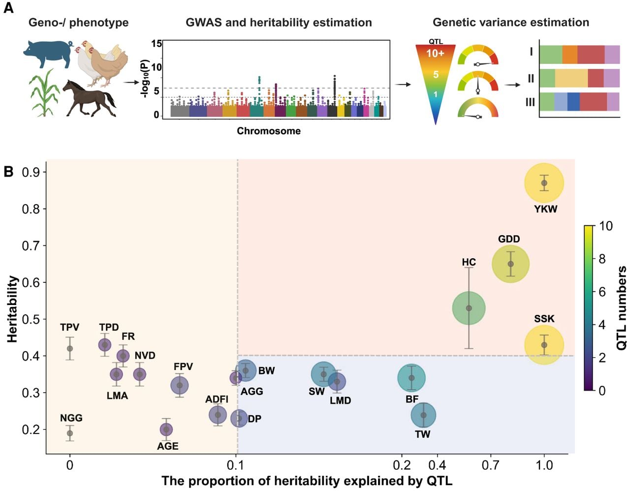
We analyzed 20 traits in six animal and plant populations (Fig. 1A). A summary of the phenotypic and genotypic data is presented in Supplemental Table S1 and the Methods section. The principle behind the selection of these traits is to encompass a diverse range of genetic architectures. Notable differences in the rate of LD decay were observed among the six populations (Supplemental Fig. S1). The heritability of the 20 traits ranged from 0.19 to 0.87 (Fig. 1B), and the additive and epistatic variance components exhibited significant differences (Supplemental Fig. S2). A GWAS was conducted for all traits (Supplemental Fig. S3). We used the Bonferroni correction to validate the significant number of independent quantitative trait loci (QTLs) associated with each phenotype and calculated the proportion of heritability explained by QTLs using a bivariate genetic relationship matrix (GRM) model. We hypothesized that the presence of effective features is a key factor influencing the accuracy of ML predictions. Based on the heritability estimates and the proportion of heritability explained by QTL, we categorized these traits into three groups (Fig. 1B): (I) high heritability effectively explained by QTLs (red; n = 4), (II) medium to low heritability effectively explained by QTLs (blue; n = 7), and (III) traits with no QTL or those that cannot be effectively explained by QTLs (purple; n = 9).
Evaluation of the genetic architecture. (A) Overview of the analytical framework. Phenotypic and genomic data from four species (pig, chicken, horse, and maize) were used to estimate heritability and genetic variance components, and a genome-wide association study (GWAS) was conducted to identify significant quantitative trait loci (QTLs). (B) Relationship between trait heritability and proportion of heritability explained by QTLs. Each circle represents a trait, and the color intensity and circle radius correspond to the number of QTLs associated with the trait. Based on heritability and the proportion of heritability explained by QTLs, traits were categorized into three categories: (I) traits with high heritability and a high proportion of heritability explained by QTLs (red; n = 4); (II) traits with moderate-to-low heritability and a high proportion of heritability explained by QTLs (blue; n = 7); and (III) traits with low heritability and a low or negligible proportion of heritability explained by QTLs (yellow; n = 9).
Comparison of the prediction accuracy of different ML methods
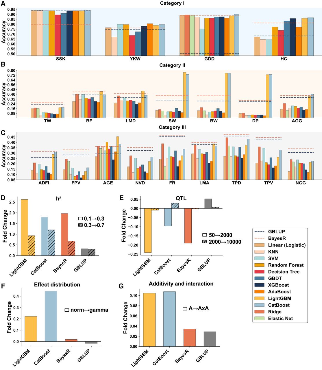
We used four categories—ordinary least squares (OLS) regression, nonlinear, bagging, and boosting—comprising 12 ML methods: linear (logistic) regression, ridge regression, elastic net, k-nearest neighbors (KNN), support vector machine (SVM), random forest, decision tree, gradient boosting decision tree (GBDT), extreme gradient boosting (XGBoost), adaptive boosting (AdaBoost), light gradient boosting machine (LightGBM), and categorical boosting (CatBoost). These methods were evaluated alongside the traditional GBLUP and BayesR methods, which served as benchmarks. The model used fivefold cross-validation to estimate the accuracy of GPs. Figure 2, A through C, and Supplemental Table S2 present the prediction accuracies of the methods across all traits. The performance of various ML methods did not show a direct correlation with the LD decay of the associated population. However, the accuracy of both the ML and traditional methods was closely related to our classification. Among the category I–type and category II–type traits, the ML methods outperformed traditional methods in 91% of cases (10 out of 11). Boosting algorithms, particularly LightGBM and CatBoost, nearly achieved optimal solutions among all the ML methods. Specifically, LightGBM yielded optimal solutions across the five traits, resulting in an average accuracy improvement of 83.15% and 32.28% compared with GBLUP and BayesR, respectively. CatBoost achieves optimal solutions across five traits and improves the accuracy by an average of 57.84% and 30.75% compared with the GBLUP and BayesR methods, respectively. In contrast, the BayesR method demonstrated superiority in 89% of the type 3 traits (eight out of nine), attributed to a rapid decline in the proportion of heritability explained by QTL. The GBLUP method did not yield the optimal results for any trait.
Prediction accuracy comparison using real and simulated data. (A–C) Real data categorized into three classes, employing GBLUP (dark blue dashed line) and BayesR (orange dashed line) as baselines for comparison with 12 machine learning (ML) methods. Some methods are unavailable for a minority of traits. The vertical axis represents results from fivefold cross-validation. (D–G) Simulated data used to evaluate how heritability (D; 0.1, 0.3, 0.7), the number of known QTLs (E; 50, 2000, 100,000), distribution of genetic effects (F; normal, gamma), and genetic models (G; additive, additive × additive) influence the accuracy of four models. The vertical coordinate represents the fold change in prediction accuracy before and after the variation of each single variable.
Evaluating the impact of parameters on different models using simulated data
To investigate the effects of various genetic parameters on different model categories, we conducted an evaluation using simulated data that included heritability values of 0.1, 0.3, and 0.7; numbers of QTLs of 50, 2000, and 100,000; effect size distributions (normal and gamma); and nonadditive effects (additive and additive × additive) (Supplemental Table S3). The ML methods employed were LightGBM and CatBoost, which demonstrated superior performance on real phenotypes. Figure 2, D through G, illustrates the results from different models, with the fold change in accuracy represented on the vertical axis. The accuracy of all four models significantly increased with higher heritability (Fig. 2D). As the number of QTLs increased from 50 to 2000, only GBLUP exhibited improved accuracy, whereas further increases in QTL numbers resulted in negligible changes across all models (Fig. 2E). When the simulated data followed a gamma distribution, both ML methods demonstrated significantly greater performance improvements compared with GBLUP and BayesR (Fig. 2F). Notably, in the presence of additive × additive interaction effects, the two ML methods also showed significant enhancements compared with GBLUP and BayesR (Fig. 2G). These findings suggest that the LightGBM and CatBoost algorithms offer considerable advantages over traditional methods when addressing genetic effects characterized by nonnormal distributions and genomic interaction effects. They also exhibit improved performance in managing traits with high heritability and well-defined QTLs.
Impact of feature selection on prediction accuracy
ML methods have demonstrated superior predictive performance for traits governed by numerous QTLs that exhibit major effects. However, this was not the case for TW (Fig. 2B). An intriguing multieffect QTL affecting both the weight of the rooster testicles (TW) and the age at which the hens begin to lay eggs (AGG) provided an opportunity to further explore the influence of features on predictions. These two traits are significant reproductive characteristics in both sexes of poultry. We identified an almost coincident QTL in the Chr 28: 1.90–2.10 Mb region (Fig. 3A). Although the total number of SNPs was comparable, the number of AGG markers within this QTL was considerably higher than that in TW (Supplemental Fig. S4). Consequently, we hypothesized that the restricted number of feature loci in the major QTL region impedes the model's ability to integrate features and develop effective branching structures, ultimately diminishing its predictive power.
The refined improvement of features impacts the prediction accuracy. (A) Manhattan plot of Chromosome 28 for AGG and TW traits. The x-axis represents the genomic position (Mb) along Chromosome 28, and y-axis denotes the −log10 P-value from the GWAS. The blue and orange points represent SNPs associated with AGG and TW, respectively. The dashed curve marks the boundaries of the significant QTL loci for both traits within this genomic interval, which encompasses multiple candidate genes, including the AMH gene. (B,C) Comparison of prediction accuracy across different models for TW and AGG traits. The column chart shows the mean prediction accuracy for the four models, and the error bars show the standard deviation of the accuracy estimates from fivefold cross-validation. (Original) Prediction using original SNP data from Supplemental Table S1, (Original+Chr28) enhancing SNP density across Chromosome 28 using sequencing data, and (Original+QTL) increasing marker density specifically within the identified QTL region on Chromosome 28. (D) Prediction accuracy of AGE and BF traits based on SLDP feature optimization strategy. The comparison includes the GBLUP, BayesR, LightGBM, and CatBoost models, as well as the two ML models combined with SLDP optimization (LightGBM-SLDP and CatBoost-SLDP).
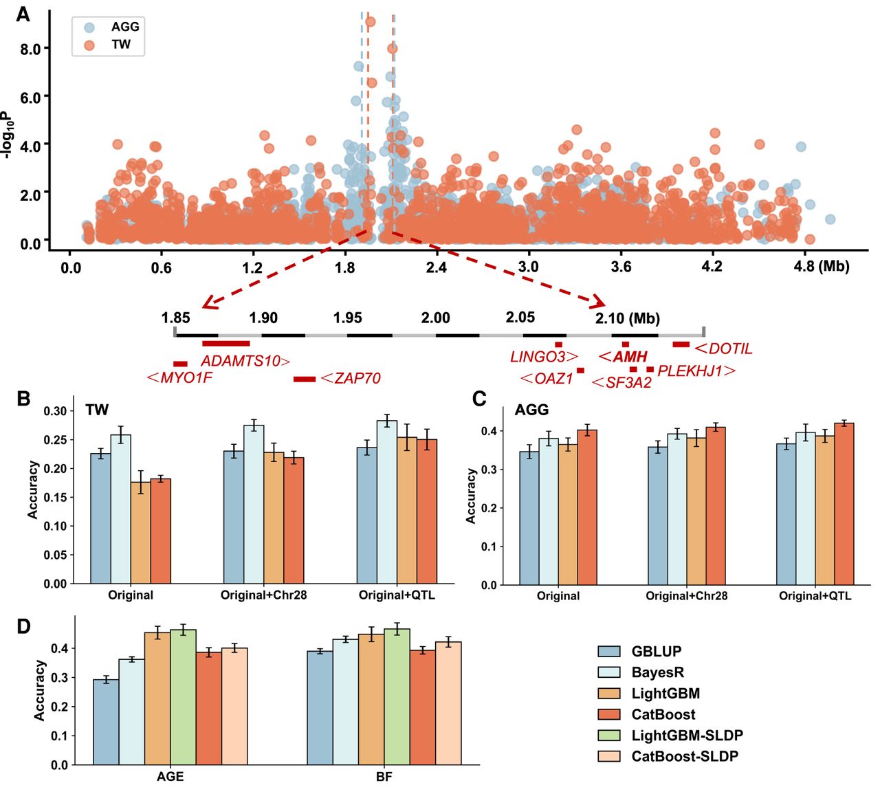
We used sequencing data to locally enhance the density of genetic features (Supplemental Fig. S4) and developed two new sets of collections: (1) increasing the marker density across Chr 28 and (2) focusing on the QTL within Chr 28. The prediction results of the four models (GBLUP, BayesR, LightGBM, and CatBoost) exhibited varying degrees of improvement. The second strategy achieved the optimal solution in all results. For TW, the accuracies of the two ML methods (LightGBM and CatBoost) were 0.2541 and 0.2503, respectively, surpassing the optimal result for GBLUP (0.2363) (Fig. 3B). Similar results were observed for AGG traits. CatBoost maintained the best predictive performance after applying the two SNP selection strategies (Fig. 3C). We applied the aforementioned strategy to the whole genome using a similar approach, SLDP (Zhu et al. 2023), to optimize the feature combination of AGE and BF. The results also showed a significant improvement (Fig. 3D). Compared with the GBLUP and BayesR methods, SLDP combined with the LightGBM strategy yielded enhancements of 58.33% and 28.06% for AGE traits and 19.56% and 5.76% for BF traits, respectively. By integrating marker selection strategies with ML methods, we can significantly enhance predictive accuracy and exploit the potential of ML models.
Parameter optimization based on the sparrow search algorithm
To further investigate the performance of the ML model improved by the search algorithm, we designed three sets of experiments: single-parameter search, grid search, and sparrow search algorithm (SSA). Here, we focused on the key hyperparameters that significantly affected LightGBM and CatBoost, including the learning rate, maximum depth, and number of leaves (Table 1). The experimental results demonstrated that single-variable tuning yielded the lowest accuracy, with unstable relative errors across the test sets, whereas Grid search exhibited marginally better stability and performance. The GA-optimized ML model outperformed both models, achieving the highest accuracy, lowest root mean square error (RMSE), and best R2, confirming its superior predictive capability and robustness. Take the TW trait as an example; by optimizing the sparrow search algorithm, the accuracy of the LightGBM and CatBoost methods reached 0.27 and 0.28, respectively. These results represent an improvement of >50% compared with the single-parameter search method and surpass those obtained with BayesR. The SSA can effectively optimize the hyperparameters of ML models, enhancing both prediction accuracy and stability and establishing it as a more competitive approach for GP tasks.
Hyperparameter optimization of different methods and the prediction performance
| LightGBM | Learning rate | Num leaves | Max depth | Min data in leaf | Feature fraction | RMSE | Pearson | Error |
|---|---|---|---|---|---|---|---|---|
| NGG | ||||||||
| Single parameter | 0.1 | 31 | −1 | 20 | 1 | 11.2 | 0.21 | 7.34 |
| Grid search | 0.05 | 15 | 3 | 30 | 0.6 | 10.67 | 0.21 | 6.94 |
| Sparrow search | 0.02 | 22 | −1 | 10 | 0.8 | 9.5 | 0.23 | 5.34 |
| AGE | ||||||||
| Single parameter | 0.1 | 31 | −1 | 20 | 1 | 4.03 | 0.45 | 3.12 |
| Grid search | 0.1 | 18 | 1 | 60 | 0.9 | 3.26 | 0.49 | 2.75 |
| Sparrow search | 0.08 | 12 | −1 | 35 | 1 | 2.94 | 0.50 | 2.01 |
| TW | ||||||||
| Single parameter | 0.1 | 31 | −1 | 20 | 1 | 9.2 | 0.17 | 7.45 |
| Grid search | 0.03 | 20 | 1 | 50 | 0.8 | 6.18 | 0.24 | 4.12 |
| Sparrow search | 0.05 | 26 | −1 | 80 | 0.6 | 4.61 | 0.27 | 3.89 |
| CatBoost | Learning rate | Depth | L2 Leaf reg | Iterations | Border count | RMSE | Pearson | Error |
|---|---|---|---|---|---|---|---|---|
| NGG | ||||||||
| Single parameter | 0.03 | 6 | 3 | 1000 | 254 | 10.32 | 0.22 | 6.21 |
| Grid search | 0.05 | 8 | 5 | 1500 | 200 | 10.13 | 0.23 | 6.06 |
| Sparrow search | 0.04 | 7 | 3 | 1200 | 86 | 9.97 | 0.24 | 5.9 |
| AGE | ||||||||
| Single parameter | 0.03 | 6 | 3 | 1000 | 254 | 6.86 | 0.38 | 5.11 |
| Grid search | 0.1 | 10 | 6 | 1300 | 64 | 5.05 | 0.43 | 4.22 |
| Sparrow search | 0.06 | 7 | 5 | 1100 | 64 | 4.78 | 0.44 | 3.76 |
| TW | ||||||||
| Single parameter | 0.03 | 6 | 3 | 1000 | 254 | 8.63 | 0.18 | 7.08 |
| Grid search | 0.06 | 10 | 5 | 700 | 64 | 5.48 | 0.26 | 3.75 |
| Sparrow search | 0.05 | 8 | 5 | 800 | 60 | 3.99 | 0.28 | 3.23 |
Interpretation of the SNP-driven ML model
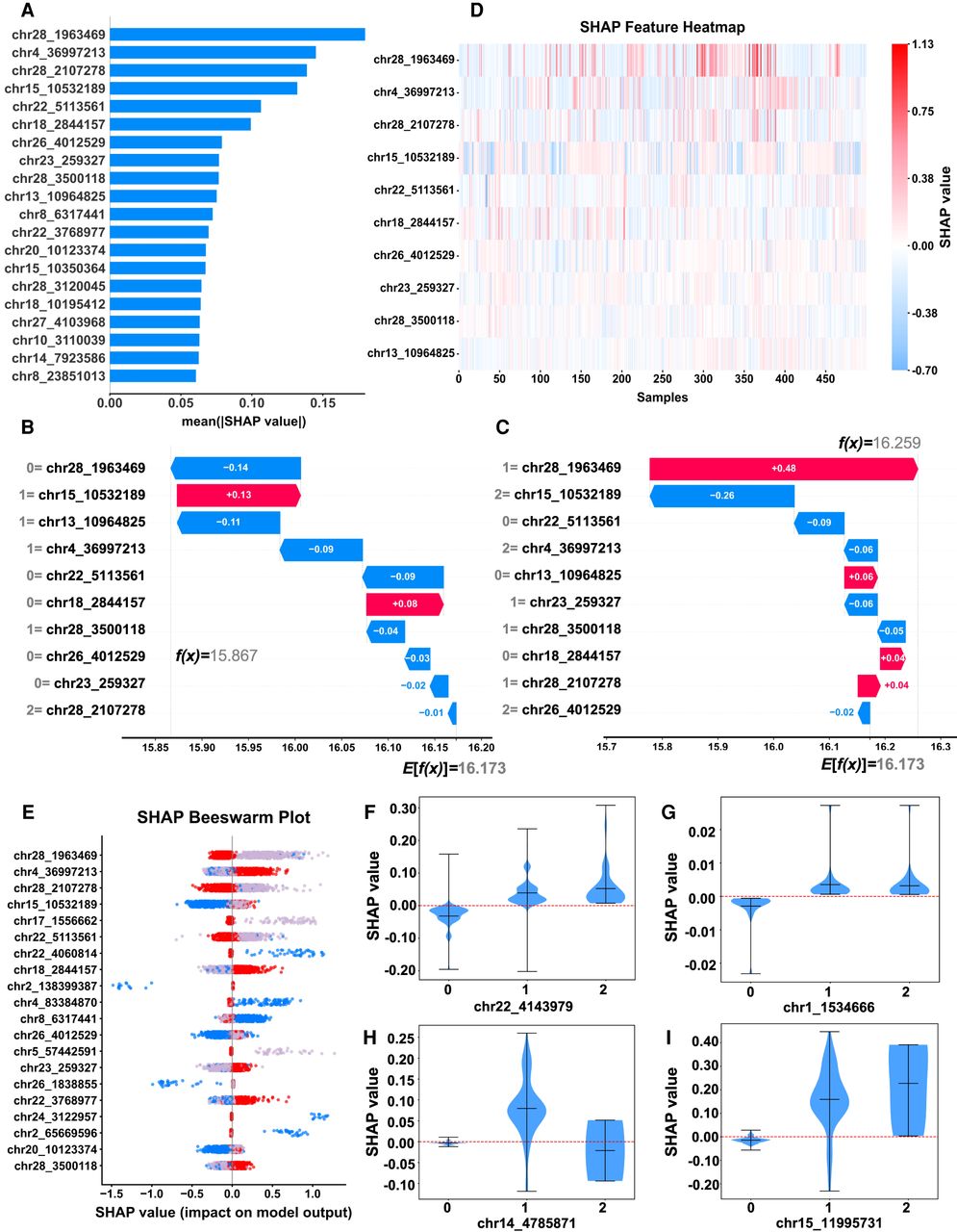
We used the SHAP method (Lundberg and Lee 2017) to interpret the ML model by quantifying each variable's contribution to predictions, taking the LightGBM model's test on the TW trait as an example. We evaluated the top 20 features via average SHAP values (Fig. 4A, presented in descending order) and found a correlation (r = 0.47) between these values and GWAS SNP P-values (Supplemental Fig. S5). The overlap rate of top SNPs between SHAP and GWAS was 60% (top five), 50% (top 10), and 70% (top 20), with major-effect loci (e.g., Chr28_1963469, Chr28_2107278, Chr22_5113561, Chr17_1556662) consistently identified, confirming high concordance in key QTL regions. Feature waterfall plots (Fig. 4B,C) illustrate individualized prediction generation: The population average prediction was 16.173, with one individual's predicted value (15.867) driven by Chr28_1963469 (genotype 0, effect = −0.14) and Chr15_10532189 (genotype 1, effect = +0.13), whereas another individual showed a higher predicted value (16.259) owing to genotype differences. Feature heatmap and beeswarm plot (Fig. 4D,E) revealed population-level SNP weight distribution, with differential SHAP values among individuals even with the same genotype. Single-site SHAP value distributions further uncovered distinct genetic patterns (additive, dominant, superdominant, epistatic) (Fig. 4F–I). Consistent interpretability patterns across traits (AGG, NGG, AGE) (Supplemental Figs. S6–S8) demonstrate that ML models effectively capture intersite interactions within populations and provide site-specific weight evaluations across independent samples.
Interpretation of the SHAP model. (A) Importance-ranking plot of SNP features. (B,C) The single-sample feature waterfall plot illustrates the SHAP values on the x-axis, and the y-axis delineates various feature values. Values 0, 1, and 2 correspond to the three genotypes AA, Aa, and aa, respectively. E[f(x)] denotes the expected value across all the samples, whereas f(x) represents the predicted value for a specific sample. (D) Heat map illustrating the distribution of features across clustered samples. The x-axis corresponds to the 500 samples, and the y-axis denotes the features. (E) Characteristic attributes in SHAP are represented on a beeswarm plot, with each line corresponding to a specific SNP feature. Genotypes are represented by different colors: AA (zero; red), Aa (one; gray), and aa (two; blue). (F–I) The distribution of SHAP values characterizes different genetic effect patterns: additive (F), dominant (G), superdominant (H), and epistatic effects (I).
Impact of dimensionality reduction on predictive performance and computational efficiency
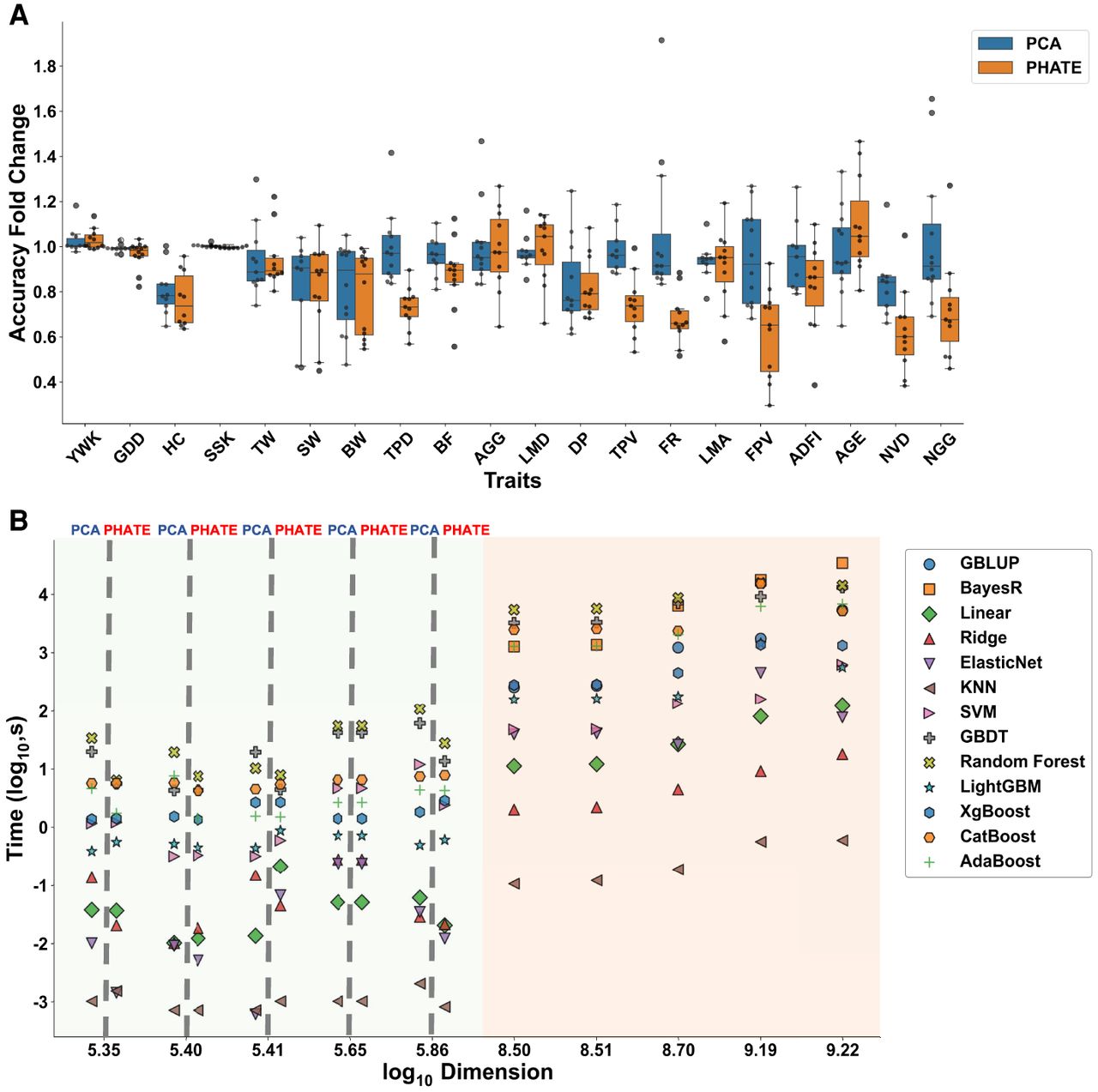
To assess the practical utility of dimensionality reduction in prediction engineering, we compared principal component analysis (PCA) and PHATE in terms of accuracy and computational efficiency. Preliminary experiments revealed no significant differences in accuracy between the 100 and 200 components in PCA and PHATE, prompting the standardized use of 100 dimensions for subsequent analyses. The fivefold cross-validation across traits (Supplemental Tables S4, S5) revealed accuracy fold changes relative to original SNP data (Fig. 5A). The average accuracy changes rates of 0.95 (PCA) and 0.85 (PHATE), with 78% of cases showing reduced accuracy, were notable for feed intake per visit (FPV) using PHATE. Certain traits, such as AGE, demonstrated improved accuracy with PHATE. The computational analysis indicates that the dimensions of the feature matrix, represented as the product of the number of samples and the number of SNPs, demonstrate a significant correlation with computation time (Fig. 5B). The original SNP data (log10 dimension > 8.36) processing required substantially longer durations (GBDT, RF, BayesR > GBLUP), whereas KNN achieved a 1000-fold faster computation. Dimensionality reduction methods reduced computation time to <2 min (a 500× speedup) across all ML models, outperforming both GBLUP and BayesR. These findings demonstrate a favorable trade-off between reduced accuracy (averaging <15%) and substantial computational savings, highlighting the practical value of dimensionality reduction in large-scale genomic analyses.
Changes in accuracy and time caused by dimensionality reduction. (A) Changes in accuracy following dimensionality reduction, with PCA represented in blue and PHATE represented in orange. The x-axis delineates various traits, and the y-axis indicates the multiplicative change in accuracy relative to the baseline accuracy obtained without dimensionality reduction. A value below one signifies that the accuracy of postdimension reduction is inferior to that of the original data set, whereas a value above one indicates an improvement. Each black point corresponds to a specific ML method, and each boxplot summarizes the distribution of accuracy changes across all ML methods applied to the corresponding trait. (B) Time comparison between different prediction methods. The y-axis denotes the logarithm of the computational duration in seconds. We calculated the logarithm of the product of the sample size and the number of SNP and plotted it on the x-axis. When the sample sizes and number of features for different traits were equal, their computational times were identical. The orange background indicates the original data set, which did not undergo dimension reduction, whereas the green background signifies the data set after dimension reduction. The PCA and PHATE results are represented on the left and right sides of the dotted line, respectively.
Design of integrated artificial intelligence software for GP
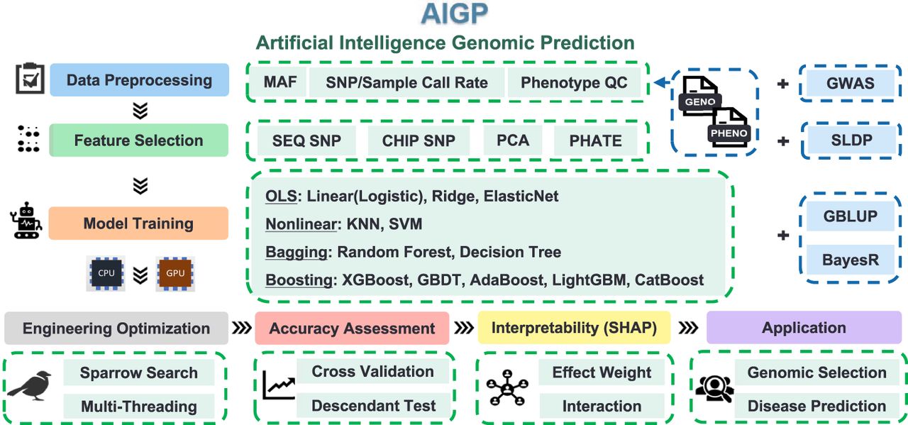
We integrated a user-friendly toolkit named artificial intelligence GP (AIGP) (Fig. 6). Specifically, AIGP begins with raw feature data that undergo preprocessing, including quality control, missing-value inspection, and multithreaded reading, ultimately converting the raw data into a format suitable for AIGP. Feature selection is an optional step performed using PCA and PHATE. Subsequently, 12 artificial intelligence models were trained to address the traits with varying genetic architectures. AIGP uses SHAP to interpret feature-effect weights, supporting both local and global analyses with visualized outputs. In addition, the toolkit integrates parameter optimization methods, including grid search, SSA, parallel computing, and multithreading, to further enhance and accelerate model performance. Users can then compare the optimal results for the target population and the traits for subsequent applications. The AIGP software includes both a command-line and a GUI-based graphical version. These materials are freely available at GitHub (see Code availability).
Overview of the artificial intelligence genomic prediction (AIGP) framework. The AIGP consists of the following: (1) data preprocessing, including SNP/phenotype quality control and integration with GWAS/SLDP; (2) feature selection, using SNP data, PCA, and PHATE; (3) model training, incorporating linear (OLS), nonlinear, and ensemble learning (bagging, boosting) methods; (4) optimization and evaluation, enhancing computational efficiency with sparrow search, multithreading, cross-validation, and SHAP-based interpretability; and (5) application, focusing on genomic selection and disease prediction.
Discussion
In this study, more than 10,000 cross-validation and combinatorial experiments were conducted using various feature optimization techniques and artificial intelligence methods. The central focus of this study was to identify the genetic parameters that significantly influenced ML predictions. By systematically evaluating multiple factors, we demonstrated that trait genetic architecture and feature selection were the primary determinants of predictive performance. These results emphasize the critical need for comprehensive characterization of genetic architectures before implementing GP strategies, as this understanding will inform optimization.
From a computational perspective, boosting algorithms (notably CatBoost and LightGBM) consistently outperformed other ML methods. CatBoost excels in processing categorical features while mitigating gradient bias and prediction shift, reducing risk (Prokhorenkova et al. 2018; Ibrahim et al. 2020). In contrast, LightGBM uses a leafwise splitting strategy that optimizes loss reduction at the terminal nodes and efficiently handles categorical variables without one-hot encoding. Parametric methods like ridge regression showed limited accuracy, likely failing to adequately account for biological batch effects. In hyperparameter optimization, the sparrow search algorithm (SSA) outperforms grid search in computational efficiency and performance (Xue and Shen 2024). SSA dynamically adjusts search directions via global–local integration, avoiding grid search's exhaustive computations to drastically reduce complexity and time, especially in high-dimensional spaces, and adapts to better capture global optima. In contrast, grid search may miss optimal parameters or get trapped in local optima. Thus, SSA is a more precise, efficient choice for large-scale hyperparameter tuning of ML models. In addition, when comparing AIGP with deep learning models such as WheatGP and Cropformer (Wang et al. 2025a,b), these methods underperformed AIGP for most traits despite their strong feature-extraction capabilities, likely owing to architectures not optimized for high-dimensional SNP data (Supplemental Table S6). However, for traits with prominent local nonlinear effects, Cropformer achieved comparable accuracy to AIGP, highlighting its potential under specific genetic architectures.
Examining ML from the perspective of genetic architecture would make for an interesting interdisciplinary discussion. Our findings revealed that traits governed by oligogenic architectures (controlled by a limited number of loci) demonstrated superior ML performance. The progressive performance improvements observed through the feature engineering suggest that even basic feature weighting strategies (Fig. 3D) can yield substantial enhancements, mirroring the feature optimization effects observed in linear modeling frameworks (Edwards et al. 2016). Moreover, handling higher-order interactions may be a scenario in which ML algorithms naturally outperform traditional methods. Traditional linear models typically represent such relationships by explicitly constructing interaction terms. However, this approach can lead to rapid dimensionality expansion and challenges in capturing potential high-order interactions. In contrast, boosting tree algorithms combine features through hierarchical conditional judgments. This mechanism inherently introduces multilevel conditional dependencies, enabling the model to automatically express nonlinear effects and potential higher-order interactions. This aligns precisely with the concept of “omnigenic” models proposed in the functional genomic era, which posits that each gene plays a synergistic role within a regulatory pathway to collectively influence complex traits (Richard et al. 2025; Zhu et al. 2025b).
The SHAP framework implemented in this study operates as a post hoc explanation system that quantifies feature contributions to model outputs through marginal effect analysis. This enables both the global and local interpretability of black-box models, generating SNP weight estimates at the individual level that account for multilocus interaction effects, which is a critical advantage over traditional mixed-linear models. Because of fundamental methodological differences between SHAP and GWAS, some loci were identified only by SHAP. These variants typically have small additive effects or low allele frequencies and thus fail to reach significance in single-marker linear models, yet they contribute substantially to phenotype through nonlinear or interaction effects in ML models. This explains the discrepancies in SNP effect prioritization between the two approaches (Supplemental Fig. S5). Evaluating SHAP interaction results across two or more sites is challenging under our current computational conditions because the computational demand scales quadratically with the number of input features, requiring significantly greater computing power.
Across all current evaluations, we did not identify a single optimal model suitable for all traits. However, we have clarified that ML algorithms will better demonstrate their potential to surpass traditional methods in scenarios involving well-defined functional sites or higher-order complex interactions. We developed AIGP, a comprehensive toolkit that integrates all evaluated AI models. Our recommended best practice is to systematically evaluate the genetic architecture of the target trait and select the optimal model based on the parameter variation cues illustrated in Figure 2. However, our software defaults to exhaustive calculations across all methods, which are computationally feasible and provide a straightforward alternative that requires no prior knowledge of the trait's genetic architecture. We also facilitated enhancements in feature engineering across various dimensions (Zhu et al. 2023; Moghaddar et al. 2019) and applied data dimensionality reduction techniques. Our framework also accepts multiomic inputs to better support downstream target phenotype prediction, an approach shown to outperform single-dimensional predictions (Sammut et al. 2022; Kaplow et al. 2023; Wang et al. 2024), making the toolkit versatile for diverse prediction tasks. Future advancements should prioritize developing more precisely weighted features for ML via (1) marker weight optimization through multiomic annotation integration (Xiang et al. 2019; Pan et al. 2023), (2) targeted experimental/meta-population designs to reduce LD interference and enable independent feature importance assessment (Wang et al. 2020; Zhu et al. 2025a), and (3) incorporation of in silico mutational landscapes (Chen et al. 2022) and gene-editing data sets. Multimodal integration will advance phenotype prediction from single-source models to large-scale pretrained models. With self-supervised learning and causal inference, large language models play a greater role in phenotype prediction, feature learning, interpretation of key genetic mechanisms, and driving progress in biological breeding and precision medicine (Ji et al. 2021; Benegas et al. 2025; Dalla-Torre et al. 2025).
Methods
Population, genotyping, and phenotyping
The data set used in this study included four species. The chicken samples included one white-feathered broiler chicken population and two yellow-feathered broiler populations. Chicken blood samples were provided by Wen's Nanfang Poultry Breeding. A low-coverage sequencing (LCS) method (Yang et al. 2021) was used to sequence all chicken samples on the MGISEQ-T7 platform (PE150 model). BaseVar version 1.01 (Liu et al. 2018) and STITCH version 2.0 (Davies et al. 2016) were used to impute genotypes. SNPs with minor allele frequency (MAF) < 0.05, call rate (CR) <0.95, and individuals with a CR <0.90 were excluded from further analyses. LD-based filtering was performed using PLINK v1.90 with specific window and step sizes and an r2 threshold. Specifically, LD pruning was conducted using a window size of 2000 SNPs and a step size of 500 SNPs across all populations. The r2 threshold was selected based on population-specific genomic features: r2 = 0.9 for Duroc pigs, r2 = 0.5 for yellow-feathered broiler chickens A and B, and r2 = 0.7 for white-feathered broiler chickens. These settings were chosen to balance redundancy and genomic coverage. After LD-based filtering, the final number of SNPs retained for each data set is listed in Supplemental Table S1. The phenotypic data of chicken were collected from Wen's Nanfang Poultry Breeding, including body weight at 90 days of age (BW), slaughter weight at 91 days of age (SW), dressed percentage (DP), egg production at 300 days of age (EGG) and age at first egg (AGG), and testicular weight at 90 days of age (TW). Individuals with phenotypes outside three standard deviations of the population mean were excluded.
Data on pig populations were obtained from a previous study (Yang et al. 2021). Ten traits were selected for our study, including age to reach 100 kg live weight (age), loin muscle area at 100 kg live weight (LMA), loin muscle depth at 100 kg live weight (LMD), and back fat thickness at 100 kg live weight (BF), average daily feed intake (ADFI), number of visits to the feeder per day (NVD), time spent eating per day (TPD), time spent eating per visit (TPV), FPV, and feed intake rate (FR). The quality control standards for the genotype and phenotype were consistent with those used in the chicken studies mentioned above. After quality control, 2549 pigs with complete growth-trait records and 2610 pigs with complete feeding behavior records were retained. The final number of SNPs used for GP was 124,679.
Maize data were obtained from a previous study (Romay et al. 2013) via genotyping-by-sequencing (GBS), yielding 681,257 SNPs across all maize lines. Phenotypic data included two case/control traits, yellow or white kernels (YWKs) and sweet or starchy kernels (SSKs), and one quantitative trait, the effective cumulative temperature (GDD). The maize data set comprised 2631 individuals for the SSK trait, 1595 for the YWK trait, and 2279 for the GDD trait.
The 480 horse samples were from the public EquineSNP50 BeadChip data set with preapplied HWE filtering (reasonable given the natural, genetically diverse population). After filtering, 50,621 SNPs remained, excluding those with a MAF of less than 0.01, a CR <0.90, and P-values < 0.001. The trait under investigation was horse color (HC), which was categorized into four classes: reddish-brown, black, gray, and silvery-white. (McCue et al. 2012). The final sample sizes and genotype information for all traits are listed in Supplemental Table S1.
Simulated data design
We conducted a comprehensive simulation experiment using the SIMER v1.0 platform (Yin et al. 2025). The major features we employed include heritability (0.1, 0.3, 0.7), number of QTLs (50, 2000, 100,000), effect size distribution (normal, gamma), and nonadditive effects (additive, additive × additive). Based on the phenotype simulated data sets (n = 5000), we compared the two ML models from our empirical study—LightGBM and CatBoost—against the traditional approaches GBLUP and BayesR. The other experimental parameters are specified as follows: in Figure 2D, QTL = 50, normal distribution, and additive model; in Figure 2E, h2 = 0.3, normal distribution, and additive model; in Figure 2F, QTL = 50, h2 = 0.3, and additive model; and in Figure 2G, QTL = 10, SNP = 10 k, normal distribution, = 0.7, and = 0.1.
Genetic architecture evaluation
LD decay curves were initially computed to analyze the differences and genetic diversity among species. The heritability of each trait was estimated using the AIREML method for variance component estimation, and the GRM was used to calculate the individual variance–covariance matrix. Epistatic mixed-model association analysis (REMMA) (Ning et al. 2018) was applied to assess the effects of various variance components across all traits. Subsequently, a GWAS was conducted for all traits, with the significance threshold adjusted using the Bonferroni correction, calculated as 0.05 divided by the number of SNPs across different populations. Based on the GWAS results for all traits, the number of QTLs was counted for each trait. Significantly associated SNPs that were located >500 kb apart were considered to belong to two distinct QTLs. A Dual GRM model was used to calculate the proportion of heritability explained by QTLs. Using these results, traits were categorized based on QTL count, heritability magnitude, and the proportion of heritability explained by QTLs, providing a refined classification of genetic structures across traits.
GP and evaluation
Given that fivefold cross-validation demonstrates similar accuracy and stability to 10-fold cross-validation (Supplemental Table S7). We used fivefold cross-validation in AIGP to assess the accuracy of the GPs. For qualitative traits, accuracy served as the evaluation metric, whereas for quantitative traits, mean squared error (MSE) was used as the loss function. Finally, the Pearson correlation coefficient between the true phenotypic values and predicted values in the candidate populations was computed over five iterations, and the average was taken as the final evaluation metric.
GBLUP and BayesR models
GBLUP is widely used in plant and animal breeding processes, and its prediction model is as follows:
The BayesR analytical methodology has been described by Erbe et al. (2012). It is assumed that SNP effects βi follow a four-component normal mixture. The effect of the SNP i was assumed to be distributed as follows:
ML model
All ML methods in AIGP are categorized into four major groups—OLS regression, nonlinear methods, bagging, and boosting—that encompass 12 models. The specific modeling principles and mathematical formulations for each category are summarized as follows. The OLS regression models included linear, logistic, ridge, and elastic net. The fundamental optimization objective for these methods was to minimize the sum of the squared errors, as shown in Equation 3:
SVM uses kernel functions to map data into a high-dimensional space. The geometric margin ri of a sample point xi to the hyperplane (w,b) is defined as Equation 4:
KNN predicts the output of a new sample based on the K-closest training samples in the input space. The predicted value in the KNN regression is given by Equation 5:
Model training and parameter optimization
In this study, we used three hyperparameter optimization methods: single-parameter tuning, grid search (GSA), and SSA. Single-parameter tuning involves adjusting one hyperparameter at a time while keeping the others fixed, making it simple but often suboptimal owing to parameter interactions. Grid search systematically evaluates all possible hyperparameter combinations within a predefined range through exhaustive search and cross-validation, ensuring comprehensive optimization but incurring high computational costs, particularly in high-dimensional search spaces.
The SSA is a new group intelligence optimization algorithm based on the behavior of sparrows in foraging and avoiding predators (Xue and Shen 2020). The population intelligence optimization has the advantages of a strong global search capability, good stability, and fast search speed. The detailed description of SSA in genome prediction can be found in the Supplemental Methods.
To further optimize the computational efficiency and predictive performance, boosting algorithms were integrated with the sparrow search optimization strategy, specifically, LightGBM and CatBoost. During parameter optimization, model performance was evaluated using MSE, RMSE, and r.
Model interpretability
In the context of GP, SHAP treats each SNP marker (coded as 0/1/2) as an independent contributor to the model output, thereby linking ML predictions directly back to the underlying genotype matrix. By calculating the contribution of each SNP locus to the prediction outcome, SHAP quantifies its impact on phenotypic variation, uncovering interactions between loci and samples within a population, as well as the roles of individuals and loci in population-level decision making.
For a given SNP j, its encoded genotype (0/1/2) for each individual is substituted into the SHAP formulation to estimate how the model prediction changes when that SNP is included or excluded from the feature subset.
The Shapely value ϕj of the feature j is calculated as follows:
The SHAP value is the contribution of each feature in the sample, and the sum of the contributions of each feature is the final prediction of the model.
Assuming that the jth feature of the ith sample is xi,j, the predicted value of the model for the ith sample xi is yi, and the mean of the target variable for all samples is ybase, the SHAP value can be expressed as
Dimensionality reduction method
Dimensionality reduction involves projecting genotype files using two methods: PCA and PHATE. PCA transforms raw data into a set of linearly independent representations in each dimension using a linear transformation. PHATE (Moon et al. 2019) is a state-of-the-art dimensionality reduction technique that captures local and global nonlinear structures using information regarding the geometric distances between data points. During the PCA and PHATE dimensionality reduction processes, the original filtered data were used as inputs, with the dimensionality M set as the target dimension, representing the number of principal components or embedding dimensions. The raw data were transformed into an “N samples × M features” matrix, which was then used to construct the sample space for further analysis.
In this study, when N exceeded 80, the explained genomic variance exceeded 90%. Based on this, we tested N = 100, 200, and 500 across pig traits to assess prediction accuracy at different scales. The results showed that the prediction accuracy was highest at N = 100; however, as M increased, accuracy declined slightly. Therefore, for all traits and methods, we standardized the analysis using M = 100.
Model time complexity evaluation
To assess the computational efficiency of the model systematically, AIGP evaluates the runtime of all traits under different dimensionality settings by comparing the pre- and postreduction feature spaces. We used the logarithm (log10) of the product of sample size and feature count as dimensionality characteristics to quantify complexity across different traits. This allowed us to statistically analyze the computation time (measured in seconds) under different dimensional scales, providing insights into the impact of dimensionality on the model training speed and computational efficiency.
Ethics approval and consent to participate
All animals used in this study were cared for, and experiments were conducted using procedures, that complied with the requirements of the animal welfare committee of agrobiotechnology of the China Agricultural University (approval SKLAB-2014-06-07).
Code availability
The software, user manual, and analysis code are available at GitHub (https://github.com/CAU-LEI/AIGP_soft.git) and as Supplemental Code.
Data access
The raw whole-genome sequencing data generated in this study have been submitted to the NCBI BioProject database (https://www.ncbi.nlm.nih.gov/bioproject/) under accession number PRJNA1198198. The summary statistics for all traits have been uploaded to Figshare (https://doi.org/10.6084/m9.Figshare.28601417) and as Supplemental Data.
Competing interest statement
The authors declare no competing interests.
Acknowledgments
We thank Jiangli Ren, Linlin Zhang, Ce Wang, Ran Song, and Ruitao Tian for their genomic sequencing and data analyses. We also thank Bingjie Li, Di Zhu, Lilin Yin, Zhenfang Wu, and Dong Lin for valuable discussions. The analysis was performed on the high-performance computing platform of the State Key Laboratory of Agrobiotechnology and the National Research Facility for Phenotypic and Genotypic Analysis of Model Animals. This study was financially supported by the Biological Breeding-National Science and Technology major project (2023ZD04064), the National Key Research & Development Program of China (grant no. 2024YFF1001500), the Chinese Universities Scientific Fund (2025TC017), and the 2115 Talent Development Program of China Agricultural University.
Author contributions: Y.Z.W. and X.X.H. supervised this project. L.W. and Y.Z.W. prepared all data sets and conducted the experiments. Z.Q.J., B.L.F., and Z.Q.X. planned and bred the animals. Y.D.Y. tested and optimized the software package. Y.Z.W. and L.W. summarized the results and wrote the manuscript. All authors read and approved the final manuscript.
Notes
[1] Supplementary material [Supplemental material is available for this article.]
[2] Article published online before print. Article, supplemental material, and publication date are at https://www.genome.org/cgi/doi/10.1101/gr.281006.125.
References
- ↵Aguilar I, Tsuruta S, Masuda Y, Lourenco D, Legarra A, Misztal I. 2018. BLUPF90 suite of programs for animal breeding with focus on genomics. In Proceedings of the 11th World Congress on Genetics Applied to Livestock Production, Auckland, New Zealand, pp. 11–16.
- ↵Alemu A, Åstrand J, Montesinos-López OA, y Sánchez JI, Fernández-Gónzalez J, Tadesse W, Vetukuri RR, Carlsson AS, Ceplitis A, Crossa J, 2024. Genomic selection in plant breeding: key factors shaping two decades of progress. Mol Plant 17: 552–578. 10.1016/j.molp.2024.03.007
- ↵Azodi CB, Tang J, Shiu S-H. 2020. Opening the black box: interpretable machine learning for geneticists. Trends Genet 36: 442–455. 10.1016/j.tig.2020.03.005
- ↵Benegas G, Albors C, Aw AJ, Ye C, Song YS. 2025. A DNA language model based on multispecies alignment predicts the effects of genome-wide variants. Nat Biotechnol 43: 1960–1965. 10.1038/s41587-024-02511-w
- ↵Chen KM, Wong AK, Troyanskaya OG, Zhou J. 2022. A sequence-based global map of regulatory activity for deciphering human genetics. Nat Genet 54: 940–949. 10.1038/s41588-022-01102-2
- ↵Daetwyler HD, Pong-Wong R, Villanueva B, Woolliams JA. 2010. The impact of genetic architecture on genome-wide evaluation methods. Genetics 185: 1021–1031. 10.1534/genetics.110.116855
- ↵Dalla-Torre H, Gonzalez L, Mendoza-Revilla J, Lopez Carranza N, Grzywaczewski AH, Oteri F, Dallago C, Trop E, de Almeida BP, Sirelkhatim H, 2025. Nucleotide transformer: building and evaluating robust foundation models for human genomics. Nat Methods 22: 287–297. 10.1038/s41592-024-02523-z
- ↵Davies RW, Flint J, Myers S, Mott R. 2016. Rapid genotype imputation from sequence without reference panels. Nat Genet 48: 965–969. 10.1038/ng.3594
- ↵Edwards SM, Sørensen IF, Sarup P, Mackay TFC, Sørensen P. 2016. Genomic prediction for quantitative traits is improved by mapping variants to gene ontology categories in Drosophila melanogaster. Genetics 203: 1871–1883. 10.1534/genetics.116.187161
- ↵Erbe M, Hayes BJ, Matukumalli LK, Goswami S, Bowman PJ, Reich CM, Mason BA, Goddard ME. 2012. Improving accuracy of genomic predictions within and between dairy cattle breeds with imputed high-density single nucleotide polymorphism panels. J Dairy Sci 95: 4114–4129. 10.3168/jds.2011-5019
- ↵Gill M, Anderson R, Hu H, Bennamoun M, Petereit J, Valliyodan B, Nguyen HT, Batley J, Bayer PE, Edwards D. 2022. Machine learning models outperform deep learning models, provide interpretation and facilitate feature selection for soybean trait prediction. BMC Plant Biol 22: 180. 10.1186/s12870-022-03559-z
- ↵He K, Yu T, Gao S, Chen S, Li L, Zhang X, Huang C, Xu Y, Wang J, Prasanna BM, 2025. Leveraging automated machine learning for environmental data-driven genetic analysis and genomic prediction in maize hybrids. Adv Sci 12: e2412423. 10.1002/advs.202412423
- ↵Ibrahim AA, Ridwan RL, Muhammed MM, Abdulaziz RO, Saheed GA. 2020. Comparison of the CatBoost classifier with other machine learning methods. Int J Adv Comput Sci Appl 11: 738–748. 10.14569/IJACSA.2020.0111190
- ↵Ji Y, Zhou Z, Liu H, Davuluri RV. 2021. DNABERT: pre-trained bidirectional encoder representations from transformers model for DNA-language in genome. Bioinformatics 37: 2112–2120. 10.1093/bioinformatics/btab083
- ↵Kaplow IM, Lawler AJ, Schäffer DE, Srinivasan C, Sestili HH, Wirthlin ME, Phan BN, Prasad K, Brown AR, Zhang X, 2023. Relating enhancer genetic variation across mammals to complex phenotypes using machine learning. Science 380: eabm7993. 10.1126/science.abm7993
- ↵Li Y, Wu F-X, Ngom A. 2018. A review on machine learning principles for multi-view biological data integration. Brief Bioinform 19: 325–340. 10.1093/bib/bbw113
- ↵Liang M, Chang T, An B, Duan X, Du L, Wang X, Miao J, Xu L, Gao X, Zhang L, 2021. A stacking ensemble learning framework for genomic prediction. Front Genet 12: 600040. 10.3389/fgene.2021.600040
- ↵Lin Q, Feng X, Li T, Pan X, Diao S, Gao Y, Yuan X, Li J, Ding X, Zhang Z. 2024. Integrating meta-analysis of genome-wide association study with pig genotype-tissue expression resources uncovers the genetic architecture for age at first farrowing in pigs. Anim Res One Health 2: 238–249. 10.1002/aro2.62
- ↵Liu S, Huang S, Chen F, Zhao L, Yuan Y, Francis SS, Fang L, Li Z, Lin L, Liu R, 2018. Genomic analyses from non-invasive prenatal testing reveal genetic associations, patterns of viral infections, and Chinese population history. Cell 175: 347–359.e14. 10.1016/j.cell.2018.08.016
- ↵Lourenço VM, Ogutu JO, Rodrigues RAP, Posekany A, Piepho H-P. 2024. Genomic prediction using machine learning: a comparison of the performance of regularized regression, ensemble, instance-based and deep learning methods on synthetic and empirical data. BMC Genomics 25: 152. 10.1186/s12864-023-09933-x
- ↵Lundberg SM, Lee S-I. 2017. A unified approach to interpreting model predictions. arXiv:1705.07874 [cs.AI]. 10.48550/arXiv.1705.07874
- ↵Lundberg SM, Erion G, Chen H, DeGrave A, Prutkin JM, Nair B, Katz R, Himmelfarb J, Bansal N, Lee S-I. 2020. From local explanations to global understanding with explainable AI for trees. Nat Mach Intell 2: 56–67. 10.1038/s42256-019-0138-9
- ↵McCue ME, Bannasch DL, Petersen JL, Gurr J, Bailey E, Binns MM, Distl O, Guérin G, Hasegawa T, Hill EW, 2012. A high density SNP array for the domestic horse and extant Perissodactyla: utility for association mapping, genetic diversity, and phylogeny studies. PLoS Genet 8: e1002451. 10.1371/journal.pgen.1002451
- ↵Meuwissen TH, Hayes BJ, Goddard ME. 2001. Prediction of total genetic value using genome-wide dense marker maps. Genetics 157: 1819–1829. 10.1093/genetics/157.4.1819
- ↵Meuwissen T, Hayes B, Goddard M. 2016. Genomic selection: a paradigm shift in animal breeding. Anim Front 6: 6–14. 10.2527/af.2016-0002
- ↵Moghaddar N, Khansefid M, van der Werf JHJ, Bolormaa S, Duijvesteijn N, Clark SA, Swan AA, Daetwyler HD, MacLeod IM. 2019. Genomic prediction based on selected variants from imputed whole-genome sequence data in Australian sheep populations. Genet Sel Evol 51: 72. 10.1186/s12711-019-0514-2
- ↵Moon KR, van Dijk D, Wang Z, Gigante S, Burkhardt DB, Chen WS, Yim K, van den Elzen A, Hirn MJ, Coifman RR, 2019. Visualizing structure and transitions in high-dimensional biological data. Nat Biotechnol 37: 1482–1492. 10.1038/s41587-019-0336-3
- ↵Moon I, LoPiccolo J, Baca SC, Sholl LM, Kehl KL, Hassett MJ, Liu D, Schrag D, Gusev A. 2023. Machine learning for genetics-based classification and treatment response prediction in cancer of unknown primary. Nat Med 29: 2057–2067. 10.1038/s41591-023-02482-6
- ↵Moser G, Khatkar MS, Hayes BJ, Raadsma HW. 2010. Accuracy of direct genomic values in Holstein bulls and cows using subsets of SNP markers. Genet Sel Evol 42: 37. 10.1186/1297-9686-42-37
- ↵Mota LFM, Fernandes GA, Herrera AC, Scalez DCB, Espigolan R, Magalhães AFB, Carvalheiro R, Baldi F, Albuquerque LG. 2020. Genomic reaction norm models exploiting genotype × environment interaction on sexual precocity indicator traits in Nellore cattle. Anim Genet 51: 210–223. 10.1111/age.12902
- ↵Mota LFM, Arikawa LM, Santos SWB, Fernandes Júnior GA, Alves AAC, Rosa GJM, Mercadante MEZ, Cyrillo JNSG, Carvalheiro R, Albuquerque LG. 2024. Benchmarking machine learning and parametric methods for genomic prediction of feed efficiency-related traits in Nellore cattle. Sci Rep 14: 6404. 10.1038/s41598-024-57234-4
- ↵Ning C, Wang D, Kang H, Mrode R, Zhou L, Xu S, Liu J-F. 2018. A rapid epistatic mixed-model association analysis by linear retransformations of genomic estimated values. Bioinformatics 34: 1817–1825. 10.1093/bioinformatics/bty017
- ↵Novakovsky G, Dexter N, Libbrecht MW, Wasserman WW, Mostafavi S. 2023. Obtaining genetics insights from deep learning via explainable artificial intelligence. Nat Rev Genet 24: 125–137. 10.1038/s41576-022-00532-2
- ↵Pan Z, Wang Y, Wang M, Wang Y, Zhu X, Gu S, Zhong C, An L, Shan M, Damas J, 2023. An atlas of regulatory elements in chicken: a resource for chicken genetics and genomics. Sci Adv 9: eade1204. 10.1126/sciadv.ade1204
- ↵Prokhorenkova L, Gusev G, Vorobev A, Dorogush AV, Gulin A. 2018. CatBoost: unbiased boosting with categorical features. arXiv:1706.09516 [cs.LG]. 10.48550/arXiv.1706.09516
- ↵Reel PS, Reel S, Pearson E, Trucco E, Jefferson E. 2021. Using machine learning approaches for multi-omics data analysis: a review. Biotechnol Adv 49: 107739. 10.1016/j.biotechadv.2021.107739
- ↵Richard D, Muthuirulan P, Young M, Yengo L, Vedantam S, Marouli E, Bartell E, Hirschhorn J, Capellini TD. 2025. Functional genomics of human skeletal development and the patterning of height heritability. Cell 188: 15–32.e24. 10.1016/j.cell.2024.10.040
- ↵Romay MC, Millard MJ, Glaubitz JC, Peiffer JA, Swarts KL, Casstevens TM, Elshire RJ, Acharya CB, Mitchell SE, Flint-Garcia SA, 2013. Comprehensive genotyping of the USA national maize inbred seed bank. Genome Biol 14: R55. 10.1186/gb-2013-14-6-r55
- ↵Sammut S-J, Crispin-Ortuzar M, Chin S-F, Provenzano E, Bardwell HA, Ma W, Cope W, Dariush A, Dawson S-J, Abraham JE, 2022. Multi-omic machine learning predictor of breast cancer therapy response. Nature 601: 623–629. 10.1038/s41586-021-04278-5
- ↵VanRaden PM. 2008. Efficient methods to compute genomic predictions. J Dairy Sci 91: 4414–4423. 10.3168/jds.2007-0980
- ↵Vergani AM, Bagnato A, Masseroli M. 2024. Predicting bovine daily milk yield by leveraging genomic breeding values. Comput Electron Agric 219: 108777. 10.1016/j.compag.2024.108777
- ↵Wang Y, Cao X, Luo C, Sheng Z, Zhang C, Bian C, Feng C, Li J, Gao F, Zhao Y, 2020. Multiple ancestral haplotypes harboring regulatory mutations cumulatively contribute to a QTL affecting chicken growth traits. Commun Biol 3: 472. 10.1038/s42003-020-01199-3
- ↵Wang P, Lehti-Shiu MD, Lotreck S, Segura Abá K, Krysan PJ, Shiu S-H. 2024. Prediction of plant complex traits via integration of multi-omics data. Nat Commun 15: 6856. 10.1038/s41467-024-50701-6
- ↵Wang C, Zhang D, Ma Y, Zhao Y, Liu P, Li X. 2025a. WheatGP, a genomic prediction method based on CNN and LSTM. Brief Bioinform 26: bbaf191. 10.1093/bib/bbaf191
- ↵Wang H, Yan S, Wang W, Chen Y, Hong J, He Q, Diao X, Lin Y, Chen Y, Cao Y, 2025b. Cropformer: an interpretable deep learning framework for crop genomic prediction. Plant Commun 6: 101223. 10.1016/j.xplc.2024.101223
- ↵Wiggans GR, VanRaden PM, Cooper TA. 2011. The genomic evaluation system in the United States: past, present, future. J Dairy Sci 94: 3202–3211. 10.3168/jds.2010-3866
- ↵Xiang R, van den Berg I, MacLeod IM, Hayes BJ, Prowse-Wilkins CP, Wang M, Bolormaa S, Liu Z, Rochfort SJ, Reich CM, 2019. Quantifying the contribution of sequence variants with regulatory and evolutionary significance to 34 bovine complex traits. Proc Natl Acad Sci 116: 19398–19408. 10.1073/pnas.1904159116
- ↵Xu Z, Lin Q, Cai X, Zhong Z, Teng J, Li B, Zeng H, Gao Y, Cai Z, Wang X, 2025. Integrating large-scale meta-GWAS and PigGTEx resources to decipher the genetic basis of 232 complex traits in pigs. Natl Sci Rev 12: nwaf048. 10.1093/nsr/nwaf048
- ↵Xue J, Shen B. 2020. A novel swarm intelligence optimization approach: sparrow search algorithm. Syst Sci Control Eng 8: 22–34. 10.1080/21642583.2019.1708830
- ↵Xue J, Shen B. 2024. A survey on sparrow search algorithms and their applications. Int J Syst Sci 55: 814–832. 10.1080/00207721.2023.2293687
- ↵Yan J, Xu Y, Cheng Q, Jiang S, Wang Q, Xiao Y, Ma C, Yan J, Wang X. 2021. LightGBM: accelerated genomically designed crop breeding through ensemble learning. Genome Biol 22: 271. 10.1186/s13059-021-02492-y
- ↵Yang R, Guo X, Zhu D, Tan C, Bian C, Ren J, Huang Z, Zhao Y, Cai G, Liu D, 2021. Accelerated deciphering of the genetic architecture of agricultural economic traits in pigs using a low-coverage whole-genome sequencing strategy. GigaScience 10: giab048. 10.1093/gigascience/giab048
- ↵Yao Z, Yao M, Wang C, Li K, Guo J, Xiao Y, Yan J, Liu J. 2025. GEFormer: a genotype-environment interaction-based genomic prediction method that integrates the gating multilayer perceptron and linear attention mechanisms. Mol Plant 18: 527–549. 10.1016/j.molp.2025.01.020
- ↵Yin L, Zhang H, Zhou X, Yuan X, Zhao S, Li X, Liu X. 2020. KAML: improving genomic prediction accuracy of complex traits using machine learning determined parameters. Genome Biol 21: 146. 10.1186/s13059-020-02052-w
- ↵Yin D, Zhang X, Yin L, Zhang H, Tang Z, Xu J, Yuan X, Zhou X, Li X, Zhao S, 2025. SIMER: an accurate and intelligent tool for simulating customizable population data across species in complex scenarios. J Big Data 12: 49. 10.1186/s40537-025-01102-z
- ↵Zhang H, Yin L, Wang M, Yuan X, Liu X. 2019. Factors affecting the accuracy of genomic selection for agricultural economic traits in maize, cattle, and pig populations. Front Genet 10: 189. 10.3389/fgene.2019.00189
- ↵Zhou X, Carbonetto P, Stephens M. 2013. Polygenic modeling with Bayesian sparse linear mixed models. PLoS Genet 9: e1003264. 10.1371/journal.pgen.1003264
- ↵Zhu D, Zhao Y, Zhang R, Wu H, Cai G, Wu Z, Wang Y, Hu X. 2023. Genomic prediction based on selective linkage disequilibrium pruning of low-coverage whole-genome sequence variants in a pure Duroc population. Genet Sel Evol 55: 72. 10.1186/s12711-023-00843-w
- ↵Zhu D, Wang Y, Qu H, Feng C, Zhang H, Sheng Z, Jiang Y, Nie Q, Chu S, Shu D, 2025a. GCRP: integrated global chicken reference panel from 11,951 chicken genomes. Genom Proteom Bioinform 23: qzaf032. 10.1093/gpbjnl/qzaf032
- ↵Zhu X, Li C, Luo C, Bai Z, Shu D, Chen P, Ren J, Song R, Fang L, Qu H, 2025b. Mapping the regulatory genetic landscape of complex traits using a chicken advanced intercross line. Nat Commun 16: 5841. 10.1038/s41467-025-60834-x
- ↵Zou Q, Tai S, Yuan Q, Nie Y, Gou H, Wang L, Li C, Jing Y, Dong F, Yue Z, 2025. Large-scale crop dataset and deep learning-based multi-modal fusion framework for more accurate G × E genomic prediction. Comput Electron Agric 230: 109833. 10.1016/j.compag.2024.109833