

Abstract
The surge in single-cell data sets and reference atlases has enabled the comparison of cell states across conditions, yet a gap persists in quantifying pathological shifts from healthy cell states. To address this gap, we introduce single-cell Pathological Shift Scoring (scPSS), which provides a statistical measure for how much a “query” cell from a diseased sample has shifted away from a reference group of healthy cells. In scPSS, the distance of a cell to its k-th nearest reference cell is considered as its pathological shift score. Euclidean distances in the top n principal component space of the gene expressions are used to measure distances between cells. The distribution of shift scores of the reference cells forms a null model. This allows a P-value to be assigned to each query cell's shift score, quantifying its statistical significance of being in the reference cell group. This makes our method both simple and statistically rigorous. The key strength of scPSS is its applicability in a “semisupervised” setting, where only healthy reference cells are known and diseased-labeled data are not provided for model training. As existing methods do not support cell-level pathological progression measurement in this setting, we adapt state-of-the-art supervised pathological prediction and contrastive models for benchmarking. Comparative evaluations against these adapted models demonstrate our method's superiority in accuracy and efficiency. Additionally, we show that the aggregation of cell-level pathological scores from scPSS can be used to predict health conditions at the individual level.
The ability to measure cellular state transitions between healthy and diseased conditions is fundamental to understanding disease mechanisms and progression. The increasing availability of single-cell data sets and large-scale reference atlases (Regev et al. 2017; Lindeboom et al. 2021) enables comparing cell states across different conditions (Nomura 2021). However, existing tools lack the capability to identify cell populations that have shifted statistically significantly from a reference state—a critical aspect for accurate disease characterization.
Current methods based on dimensionality reduction (Kobak and Berens 2019; Xiang et al. 2021) and machine learning (Lotfollahi et al. 2022; Michielsen et al. 2023) can effectively classify cells into known states but cannot quantify the degree of shift from a reference state. Linear models using principal component (PC) embeddings of gene expression are popular for single-cell analysis, with distances in PC space being used to cluster cells into groups (Fa et al. 2021) and measure differences between these groups (Nicol et al. 2024). Furthermore, contrastive methods (Abid et al. 2018; Gorla et al. 2023) and contrastive learning approaches (Weinberger et al. 2023) have been developed to identify specific features that are more informative in distinguishing between cell groups through targeted dimensionality reduction. Whereas these approaches have improved disease-specific feature identification, they do not provide a quantitative assessment of state alterations and lack the ability to measure the degree of disease-associated changes. Recent weakly supervised machine learning methods have enabled the identification and scoring (Goeva et al. 2024; Litinetskaya et al. 2025; Wehbe et al. 2025) of disease-relevant cellular states. Among them, scIDIST (Wehbe et al. 2025) integrates autoencoder-based dimensionality reduction with weak supervision, producing probabilistic disease labels. The labels are then used to train a neural network that assigns continuous disease progression scores to individual cells. Although these methods can assign pathological scores at the single-cell level, they require labeled training data from both healthy and diseased individuals, limiting their applicability to well-characterized conditions.
To address the need for a computational method for quantifying the significance of cellular state deviations from a healthy reference, we introduce single-cell Pathological Shift Scoring (scPSS). scPSS uses gene expression profiles from normal cells to establish a reference state distribution, using k-nearest neighbor distances in principal component embedding space. For any query cell, it calculates a “pathological shift score” that measures its deviation from this healthy state distribution. This score enables both the ranking of cells by their degree of state deviation and the identification of disease progression. The key differentiator for scPSS is its semisupervised reference-based design—quantifying pathological shifts using only healthy reference distributions, without requiring training on condition-labeled data. Because scPSS does not require annotated disease data sets, it is uniquely applicable to rare and emerging diseases. Furthermore, it employs a low-parameter yet robust statistical framework that provides an intuitive measure of cellular state changes, in line with the principle of Occam's Razor. In this study, we present scPSS and evaluate its performance across diverse data sets, highlighting its effectiveness in ranking pathological shifts without the need for disease-labeled data.
Results
Overview of scPSS
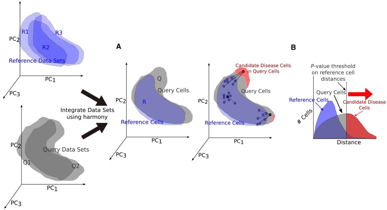
In scPSS, we find the pathological shift score of a query cell using the distance to its k-th nearest reference cell. The Euclidean distances between cells are measured in a lower-dimensional embedding of the gene expression values in order to better capture the latent biological representations. We have used principal component analysis (PCA) to get the latent representations. As a preprocessing step, the principal component projection values are adjusted using Harmony (Korsunsky et al. 2019) to account for the batch-specific differences between the different data sets. scPSS is run separately on each major cell type cluster so that the top principal components capture pathological variation rather than dominant cell type differences. This requires a cluster-to-cluster correspondence between the query and reference data sets. When cluster annotations are not available, the data sets first need to be clustered into major cell types, and the resulting clusters should then be mapped across data sets before applying scPSS.
For the statistical significance of the pathological shift scores, we first prepare a null distribution of distances of reference cells from their k-th nearest neighbor. Then, the P-value of the distance of the query cells from their k-th nearest neighbor, that is, their pathological shift score belonging to the null distribution, is determined. To ensure a continuous P-value measure for query shift scores, we fit a continuous probability distribution function to the reference shift scores. Query cells with a P-value lower than a threshold are labeled as pathological.
The number of principal components n, the k parameter for the k-th nearest neighbor used for distance calculation, and the P-value threshold for labeling query cells as pathological are obtained through a parameter selection process that maximizes outlier detection, while limiting false positives. To control for false-positive detection of significant shifts, we apply Storey's q-value method (Storey 2002).
To find pathological shifts in data sets with multiple cell types, the method compares only those cell types present in both the reference and query. To derive individual-level or sample-level pathology measures, we aggregate the shift scores of cells from each of the compared cell types. Figure 1 shows the scPSS pipeline. Further details can be found in the Methods section.
Overview of scPSS. (A) At first, the query (Q1, Q2) and reference data sets (R1, R2, R3) are concatenated together, and then principal component analysis is done. The concatenated data sets are then integrated using the Harmony method. This removes batch-specific effects on these data sets by adjusting the principal component (PC) values. (B) The Euclidean distance of a cell to the k-th nearest reference cell in PC space is used as its pathological shift score. The distances of the reference cells to their neighboring reference cells are considered as the null distribution. We can determine the P-value of each query cell distance belonging to the reference null distribution to get a significance measure for pathological progression. Cells with P-values below a specified threshold are considered significantly pathological.
scPSS identifies damaged cells and damage progression in mouse infarcted heart tissue
We validated scPSS using single-cell transcriptomic data from mouse hearts before and after myocardial infarction (MI) (Calcagno et al. 2022). The data set contains labeled cardiomyocytes (CMs) from three distinct regions: the remote zone (RZ), far from infarction, border zone 1 (BZ1), and border zone 2 (BZ2), both adjacent to infarction regions (Fig. 2A). Pre-MI samples predominantly contain RZ cells, whereas post-MI samples include a mixture of RZ, BZ1, and BZ2 cells, providing an ideal benchmark data set for testing how well different methods predict outlier disease cells using healthy cells as reference (Fig. 2B).
scPSS for damage progression in infarcted heart tissue. (A–C) The PC embeddings of all the cells from both healthy (before infarction) and query (after infarction), colored according to regions of nearness to infarcted regions (A), according to whether they belong to the reference or query data set (B), and the shift score assigned by scPSS (C). (D,E) The receiver operating characteristic (ROC) (D) and precision-recall (E) curves for the pathological scores provided by our method on the query data set. (F) Shift score distribution of reference cells with reference cells and query cells with reference cells. (G) The PC embeddings of all the cells from both healthy (before infarction) and query (after infarction), colored according to disease condition labels provided by scPSS. (H) The confusion matrix of the true labels and predicted labels given by scPSS framework on the query cells. (I) Shift score distribution of reference cells with reference cells and remote zone (RZ), border zone 1 (BZ1), and border zone 2 (BZ2) query cells with reference cells in histograms and box plots. (J) Top 30 differentially expressed genes across cells predicted pathological from query data set and reference cells. (K) The top Venn diagram shows the overlap between the DEGs reported by the original authors and those identified between predicted disease and reference cells using scPSS. The bottom Venn diagram shows the overlap between DEGs from the ground truth BZ1/2 versus RZ comparison and those from the predicted disease versus reference comparison.
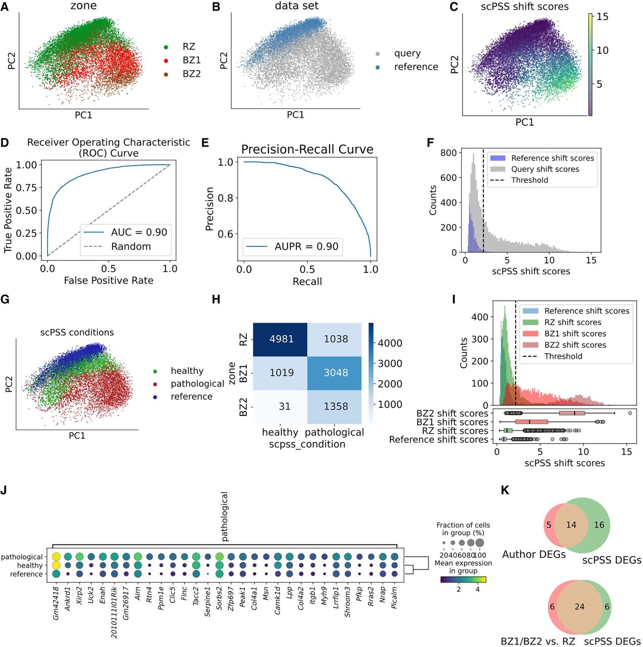
We first found the pathological scores of query cells using scPSS (Fig. 2C). These shift scores distinguished healthy (RZ) versus pathological (BZ1 and BZ2) cells with an area under the receiver operating characteristic curve (AUC) of 0.90 and the area under the precision-recall curve (AUPR) of 0.90 (Fig. 2D,E). After computing shift scores, scPSS determines an optimal threshold that best separates the reference and query distributions. This threshold is then used to classify query cells as healthy or pathological (Methods; Fig. 2F,G). To further reduce false positives, Storey's q-value false discovery rate correction is applied: query cells with q > 0.15, corresponding to a positive false discovery rate of 15%, are considered likely false positives and reclassified as healthy. For the case where pre-MI cells are used as reference and post-MI cells at all time points as query, scPSS was able to classify RZ cells as healthy and BZ1 and BZ2 cells as diseased at an accuracy of ∼81% (Fig. 2H). We also found that the scPSS scores of BZ2 from the reference were more than the scores of BZ1 (Fig. 2I).
Furthermore, classifying the query cells enabled us to identify disease-associated genes through differential expression analysis between the predicted pathological and reference cell populations (Fig. 2J). The original authors reported 31 differentially expressed genes (DEGs) of CMs across different regions. Among these, 19 were present in all pre- and post-MI samples. Of those 19, 14 were also found among the top 30 DEGs identified in the comparison between predicted pathological and reference cells. Also, 24 of the top 30 differentially expressed genes identified between ground truth BZ1/BZ2 and RZ cells were also found among the top DEGs obtained between predicted pathological and reference cells (Fig. 2K).
The scPSS method picks the k parameter, used for k-th nearest neighbor distance, through parameter optimization for each reference and query data set pair. This adaptive design helps mitigate the sensitivity of pathological rankings to variations in data set sizes (i.e., the number of cells) in both the query and reference data sets. To validate this, we evaluated the AUC and AUPR of scPSS when identifying diseased (BZ1 and BZ2) cells from post-MI data sets while using pre-MI data sets as reference, under different subsampling conditions. When both the reference and query data sets were subsampled to 500 cells, or when only the reference was subsampled, there was no degradation in median AUPR. When only the query data set was subsampled to 500 cells, the median AUPR decreased by only 1.61% (Supplemental Fig. S3). These results indicate that the pathological rankings remained stable, unless the data set size was greatly reduced (number of cells < 500), indicating that scPSS is robust to data set size variation. Furthermore, because our method provides P-values for pathological shifts, these offer a more consistent means of measuring and comparing shifts across reference-query data set pairs of varying sizes.
During parameter optimization, we allowed a minimum disease P-value threshold of 0.10. This means that up to 10% of the reference cells could be labeled as pathological by design. Also, in all of our analyses, we have consistently allowed for a false discovery rate of 15% (q-value < 0.15). Therefore, even without disease cells, around 15% of false-positive results in the query can be expected. To assess the false positive rate of our procedure, we applied scPSS to healthy control data sets used as queries against other healthy reference data sets. In the original data set, there were three healthy samples. In each of the three negative control settings, we used one healthy sample as the query and the remaining two as references. The resulting false positive rates were 8.0%, 0.1%, and 20.3% on the three settings. In these same settings, we also observed that 7.6%, 0.1%, and 13.8% of the reference cells’ shift scores exceeded the pathological (p- and q-value) thresholds, meaning they, too, were marked as pathological (Supplemental Fig. S4). If we compare the differences between the ratio of cells beyond the pathological threshold in the query and reference cells from the positive diseased settings (query is diseased) and the negative control settings (query is healthy), we find the difference to be much larger in the problem scenarios where there are diseased cells in the query data set (Cohen's d > 70) and the negative control scenarios (Cohen's d < 10). These results demonstrate that, in the negative case control setting, scPSS maintains a low false positive rate, near the allowed FDR rate, and a low difference in outlier ratios between reference and query. The outliers detected in negative control settings are likely from sample-specific technical variations.
By design, the scPSS framework is flexible and supports multiple options for dimensionality reduction, integration methods, and point-to-point distance metrics. Comparisons across different methods show that, keeping all other components constant, replacing PCA and Harmony with PCA and Scanorama or scVI for dimensionality reduction and integration degrades performance (Supplemental Tables S1–S3). Similarly, comparisons across various distance metrics indicate that Chebyshev, Euclidean, MSE, and Minkowski perform the best, whereas metrics such as Bray–Curtis and Cosine show poorer performance (Supplemental Tables S4, S5).
scPSS classifies the condition of individuals from pathological cell proportions
We evaluated scPSS's ability to classify disease states at the individual level using a subset of the Human Lung Cell Atlas (HLCA) (Sikkema et al. 2023) that has been used in the study by Litinetskaya et al. (2025), containing single-cell data from 59 healthy individuals and 52 patients with idiopathic pulmonary fibrosis (IPF). Using the pathological progression scores of each individual cell, it is also possible to provide the pathological labels of each individual organism/specimen (Fig. 3A). In this context, we are evaluating the accuracy of correctly classifying query individuals as healthy or diseased based on their cell-level pathological scores. scPSS provides a pathological score for the query cells and a threshold above which a query cell can be considered as pathological (Fig. 3B). These pathological labels are corrected for false positives with Storey's q-value method with a q threshold of 0.15. The individual is labeled as healthy or diseased depending on the proportion of pathological cells of different cell types in an individual. Individuals in the query data set with significantly higher pathological proportions than reference healthy individuals are considered to be diseased (Fig. 3C; Methods).
scPSS predicting healthy versus IPF. (A) Schematic diagram of predicting individual pathological condition using scPSS: At first, we find the pathological scores of each individual cell for the query individual by comparing against healthy references using scPSS on each individual cell type. Then, we aggregate these scores to get the individual's final pathological score. (Parts of the image have been adapted from SVG Human With All Organs.svg, which is under the CC BY-SA 3.0 license.) (B) Distance distribution of reference cells with reference cells and query cells with reference cells for the macrophage cell type in one example fold. (C) Violin plots of outlier ratios or disease ratios of reference and query individuals for the macrophage cell type in one example fold. (D) With only healthy cells present in the reference data set, the accuracy of scPSS pipeline at predicting healthy versus IPF condition of individuals based on the proportion of pathological cells of each cell group and all cells together. (E) With cells from both healthy and diseased individuals in the reference data set, we see an increase in predictive accuracy for the same experiment. (Note: For calculating accuracy for a certain cell type, we considered only the individuals with cells of that type.)
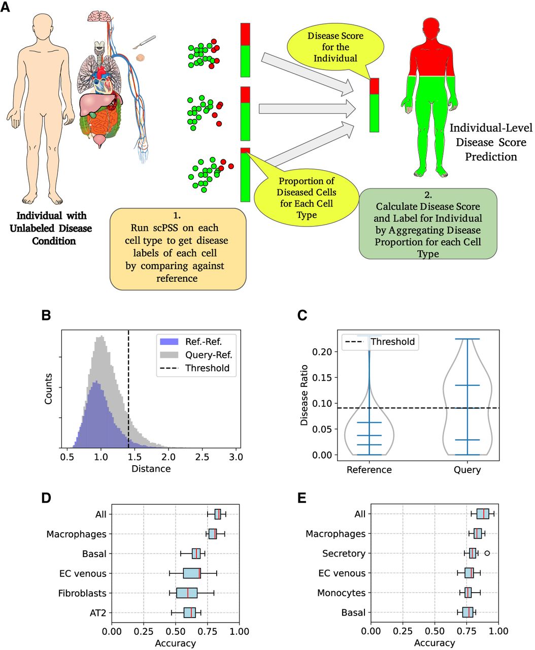
In our first experiment, we used healthy reference data only, randomly selecting 50% of healthy individuals as reference and the remaining healthy individuals plus 50% of IPF patients as query samples. This problem setup reflects the scenario when we have cell samples from healthy individuals as reference and need to classify individuals as healthy and diseased. To ensure robust evaluation, we repeated this procedure 10 times with different random choices of individuals into reference and query sets. When only the pathological proportions of individual cell types were used for classification, we found that macrophages alone achieved a median classification accuracy of ∼81%. Other cell types, basal, endothelial cells of venous type (EC Venous), fibroblasts, and alveolar type 2 (AT2) clusters, were also found to be strong indicators of disease state. When we considered the disease portions of these five cell types together, we achieved a median accuracy of ∼84% with minimum-2 outlier voting aggregation (Methods; Fig. 3D).
If we have both healthy and diseased individuals in our reference data set, we can better predict healthy and diseased individuals in the query data set (Methods). To show this, we repeated the same experiment. However, this time, we randomly picked 50% of the healthy individuals and 50% of the diseased individuals into the reference data sets and the rest into the query data set. In this setting, we have found the disease proportions of cell types: macrophages, secretory, EC venous, monocytes, and basal, to be the best predictors of individual pathology. Using average disease proportion (Methods) of the five indicative cell types, we have found the accuracy to be ∼88% (Fig. 3E). We compared which cell types have the greatest total shift by comparing the shift scores by using the cells from healthy individuals as reference and those from IPF patients as query. Among the major cell types (with cell count > 5000), we found EC venous, fibroblasts, secretory, macrophages, basal, and AT2 to have the greatest shifts (Cohen's d > 0.5). These results are broadly consistent with previous reports that highlight the central roles of fibroblasts, macrophages, and epithelial cells (particularly AT2 and aberrant basal-like cells) in IPF pathogenesis (Adams et al. 2020; Habermann et al. 2020). From our analysis, we also found that mature lymphatic endothelial cells (lymphatic EC mature), natural killer cells of the innate lymphoid lineage (innate lymphoid cell NK), multiciliated epithelial cells (multiciliated lineage), and B lymphocytes (B cell lineage cells) have comparatively lower shifts (Cohen's d < 0.2) (Supplemental Fig. S5).
scPSS identifies pathological progression in BMMC of leukemia patients
We applied scPSS to analyze bone marrow mononuclear cells (BMMC) from leukemia patients before and after bone marrow transplantation (Zheng et al. 2017). From this data set, we used cells from two healthy donors as our reference and cells from two patients with acute myeloid leukemia (AML) before and after undergoing hematopoietic stem cell transplantation (HSCT) as our query data sets to check the pathological progression of cells in pretransplant and posttransplant conditions. We ran scPSS in two modes: (1) on all the cell types together; and (2) separately for each cell type. Cells were clustered into their cell types and annotated as discussed in the Methods section.
When scPSS was applied to all the BMMC cells together, we allowed for larger values of k during parameter selection (see Methods for parameter selection). The optimal k value was selected as 500 by automatic parameter estimation. This large k-value makes scPSS capture distance from the global distribution, instead of local variation. So, here, scPSS is detecting variations in the proportion of cell types rather than shifts within each cell type. The scPSS scores of T and B cells were found to be the lowest, and those of erythrocytes were found to be higher. This suggests that the proportion of T and B cells was higher in the reference healthy group and lower in the query transplant group. In contrast, the opposite was true for erythrocytes, which aligns with the findings from the original paper (Zheng et al. 2017). scPSS showed that cells from pretransplant patients (74% with a P-value = <0.10) were more pathological than those from posttransplant cells (34% with a P-value < 0.10). This reduction in pathological cells corresponds to the reversal of the proportion of the cell type to its healthy condition following transplantation. This aligns with expected clinical recovery patterns as described by the original paper and demonstrates scPSS's utility in monitoring treatment response.
We next applied scPSS individually for each cell type. In these cases, we allowed the automatic parameter selection to search for k-values ≤ 50 (which is the default in our method). We found a reversal of pathological proportions in posttransplant patients in the case of erythroids. For the T cells, we found the pathological proportion to be higher in the posttransplant condition than in the pretransplant condition. (Supplemental Fig. S6).
Benchmarking against state-of-the-art models from related domains adapted for pathological shift scoring
To benchmark scPSS, we adapted three strong models from related domains for pathological shift scoring in the semisupervised setting: ContrastiveVI (Weinberger et al. 2023), HiDDEN (Goeva et al. 2024), and MultiMIL (Litinetskaya et al. 2025).
In contrastive learning, the goal is to learn salient representations by bringing embeddings of similar examples (positive pairs) closer together while pushing apart dissimilar examples (negative pairs). ContrastiveVI is a contrastive deep generative model that adapts this principle to single-cell data by separating condition-specific variation from shared biological variation through two distinct sets of latent features: one shared across all cells and another specific to the condition of interest. In this formulation, the “target” refers to cells from the condition of interest whose unique features we aim to identify (e.g., diseased or treated), whereas the “background” consists of control cells used as a reference for comparison. During training, the salient condition-specific latent features are fixed to zero for the background cells. This ensures that only the target cells contribute to this salient latent space. As a result, this salient latent space captures variation that is uniquely enriched in the target condition. For our problem setting, we adapted the ContrastiveVI by training it using healthy reference cells as the background and query cells as the target, so that the salient features reflect disease-specific signals. We also extended the model's utility to measure the degree of deviation of each query cell from the reference using the salient latent representations, by introducing two quantitative scoring strategies, referred to as variants 1 and 2 (see Methods).
HiDDEN and MultiMIL are weakly supervised methods that infer cell-level relevance using only sample-level disease condition labels. Both aim to link overall disease status to individual cells without requiring per-cell annotations. HiDDEN projects cells into a lower-dimensional space and trains a classifier on sample-level labels to produce per-cell perturbation scores, which are then clustered into affected and unaffected groups. MultiMIL also transforms the gene expressions into a lower dimension and then uses attention-based multiple-instance learning, where each cell receives an attention weight based on its contribution to the sample's classification. In our “semisupervised” setting, HiDDEN and MultiMIL received only sample-level labels indicating whether a sample belonged to the reference or query group. We trained HiDDEN using these labels and interpreted its per-cell perturbation scores as pathological shift scores. For MultiMIL, we used the learned attention weights as cell-level indicators of disease relevance.
For our benchmark tests, we used pre-MI (day 0) samples as the reference data set and post-MI samples as query data sets, with RZ cells representing the healthy state and BZ1 and BZ2 cells representing the diseased state. In the first benchmark setup, we used all pre-MI samples as the reference and all post-MI samples as the query. We compared the pathological scores obtained from scPSS against those from the modified ContrastiveVI, HiDDEN, and MultiMIL models (Supplemental Fig. S1) in classifying healthy (RZ) versus pathological (BZ1 and BZ2) cells, using area under the receiver operating characteristic curve and the area under the precision-recall curve metrics. The AUC and AUPR achieved by scPSS were at least 9.97% higher than those from the other methods (Supplemental Fig. S2).
We repeated this comparison 25 times to account for the variability of performance of machine learning models with differing seeds. We also performed the comparison with different query setups: using the same pre-MI samples as reference and samples from individual post-MI time points (1 h, 4 h, 1 day, 3 days, and 7 days) as query. These timepoint-specific benchmarks were also repeated 25 times per setup. scPSS outperformed the other models in all the benchmark setups (Tables 1, 2), demonstrating its superior ability to rank cells based on their deviation from the healthy reference state. In addition to the models shown in Tables 1 and 2, we also benchmarked scIDIST. But in our experiments, we found the results to be almost random (AUROC = ∼0.51).
Comparison of AUC measures between the adapted ContrastiveVI (variant 1 and 2) models, MultiMIL, HiDDEN, and scPSS (our method) for predicting healthy and damaged cells, using pre-MI (myocardial infarction) data set as reference and cells collected at different time points after MI as query data set
| Query data set | Adapted ContrastiveVI (Variant 1) | Adapted ContrastiveVI (Variant 2) | HiDDEN | MultiMIL | scPSS (Ours) |
|---|---|---|---|---|---|
| 1 h | 0.6664 ± 0.0706 | 0.5801 ± 0.0128 | 0.5031 ± 0.0000 | 0.7809 ± 0.0428 | 0.9176 ± 0.0015 |
| 4 h | 0.8295 ± 0.0670 | 0.5027 ± 0.0201 | 0.5977 ± 0.0000 | 0.9328 ± 0.0091 | 0.9403 ± 0.0006 |
| Day 1 | 0.8974 ± 0.0089 | 0.6474 ± 0.0129 | 0.6432 ± 0.0000 | 0.8444 ± 0.0325 | 0.9509 ± 0.0002 |
| Day 3 | 0.6372 ± 0.0375 | 0.5824 ± 0.0162 | 0.5396 ± 0.0000 | 0.8479 ± 0.0236 | 0.9322 ± 0.0006 |
| Day 7 | 0.6413 ± 0.0271 | 0.6668 ± 0.0060 | 0.6929 ± 0.0000 | 0.6181 ± 0.0506 | 0.8511 ± 0.0027 |
| All post-MI | 0.8114 ± 0.0350 | 0.7281 ± 0.0110 | 0.7359 ± 0.0000 | 0.7990 ± 0.0413 | 0.9012 ± 0.0004 |
[i] Results show mean ± 95% confidence interval from 25 independent runs. For each setup, the best result is highlighted in bold.
Comparison of AUPR measures between the adapted ContrastiveVI (variant 1 and 2), MultiMIL, HiDDEN, and scPSS (our method) for predicting healthy and damaged cells, using pre-MI (myocardial infarction) data set as reference and cells collected at different time points after MI as query data set
| Query data set | Adapted ContrastiveVI (Variant 1) | Adapted ContrastiveVI (Variant 2) | HiDDEN | MultiMIL | scPSS (Ours) |
|---|---|---|---|---|---|
| 1 h | 0.5369 ± 0.0747 | 0.4562 ± 0.0117 | 0.3801 ± 0.0000 | 0.6230 ± 0.0346 | 0.8426 ± 0.0033 |
| 4 h | 0.8635 ± 0.0552 | 0.6230 ± 0.0132 | 0.6685 ± 0.0000 | 0.9597 ± 0.0038 | 0.9591 ± 0.0004 |
| Day 1 | 0.9074 ± 0.0109 | 0.7169 ± 0.0097 | 0.6494 ± 0.0000 | 0.8782 ± 0.0254 | 0.9591 ± 0.0002 |
| Day 3 | 0.5099 ± 0.0405 | 0.4875 ± 0.0157 | 0.4238 ± 0.0000 | 0.7219 ± 0.0282 | 0.8944 ± 0.0011 |
| Day 7 | 0.5676 ± 0.0282 | 0.6009 ± 0.0069 | 0.5957 ± 0.0000 | 0.5611 ± 0.0408 | 0.8239 ± 0.0040 |
| All post-MI | 0.8088 ± 0.0374 | 0.7306 ± 0.0102 | 0.6825 ± 0.0000 | 0.7609 ± 0.0367 | 0.9024 ± 0.0003 |
[i] Results show mean ± 95% confidence interval from 25 independent runs. For each setup, the best result is highlighted in bold.
Discussion
In this work, we developed scPSS for pathological shift detection under a new problem setup: a semisupervised setting where reference cells are known to be healthy and the query data set is unlabeled. scPSS provides a fast but accurate statistical method for measuring pathological shifts of cells from a reference cell by using distance measures in the principal component space of gene expression values. There may be a complex, nonlinear mapping between genotypical and phenotypical space, which cannot always be captured by the linear PC embeddings. However, the linear modeling choices in scPSS, such as using PCA and Euclidean distance, were deliberate. In the absence of clearly labeled diseased cells, attempting to learn more complex embedding or distance functions risks overfitting to irrelevant patterns and failing to identify true disease states. The simplicity of scPSS serves as a form of regularization, reducing the chance of spurious findings.
Standard preprocessing steps, including filtering low-quality cells and genes, and handling dropout, should be applied before using scPSS. Failure to do so may lead to erroneous results, both for scPSS and other alternate methods. Whereas these preprocessing steps are critical for ensuring and assessing data quality, they are well-established in the single-cell analysis community and have not been further discussed in this study. scPSS requires a mapping of cell type labels between the reference and query data sets, as it ideally works on one cell cluster at a time. When annotations are missing or difficult to obtain, especially in diseased samples, the preprocessing pipeline can work around by first clustering cells into major cell types (Traag et al. 2019) and then mapping major clusters (Huizing et al. 2022) across the data sets before applying scPSS (e.g., using methods like those in Xu et al. 2021). In addition, scPSS assumes the availability of a well-defined healthy reference, which may limit its applicability in exploratory settings where such a reference is not available.
Distinguishing biological signals from technical artifacts remains a key problem in single-cell analysis, and scPSS is no exception. Batch effects, present in most data sets, can obscure changes that are disease-causing. scPSS employs Harmony for batch effect removal. However, this process may potentially remove some disease-related variation along with the technical noise, particularly when the proportion of diseased cells is unknown.
scPSS uses a parameter selection strategy to determine settings such as the number of principal components and the P-value classification threshold. These settings are chosen to maximize the detection of pathological cells while limiting false positives. As shown in our analysis, scPSS is most effective when the query data set includes pathological cells. When pathological cells are absent from the query, we found scPSS classifies up to ∼20% of query cells as pathological when used with a q-value of 0.15. Such findings with low positives should be interpreted with caution, as they may reflect false positives arising from technical artifacts rather than true pathological signals. In these cases, validation is recommended through follow-up analysis. For example, one can conduct differential gene expression and pathway enrichment analyses between predicted pathological cells and control cells to confirm that the results are biologically meaningful. If not, then the user can repeat scPSS using a different cutoff for the P-value threshold. This iterative refinement approach is common in other single-cell analysis methods, such as clustering and the detection of rare cell clusters. One iteratively refines clustering parameters, including the number of principal components to define the clustering space and the resolution, by checking if the differentially expressed genes (cluster markers) are biologically meaningful (Luecken and Theis 2019). Although scPSS provides a recommended P-value threshold, determining the cutoff point for classifying the query cells as diseased based on the pathological shift score is still a choice left up to the user. In addition, scPSS allows the user to choose a q-value for controlling false positives at different rates.
We also note the limitations that point to opportunities for future work. Although we have shown that good accuracy can be obtained using different aggregation strategies, we did not propose a general strategy or provide guidance on selecting the optimal one. In addition, because we did not find methods that are specifically designed for the semisupervised setting, we adapted approaches from related problems using simple modifications for benchmarking with scPSS. Our aim in this comparison is not to claim that existing contrastive or weakly supervised methods fail at the tasks for which they were designed. Rather, we evaluate whether minimal repurposing of such methods is sufficient for the specific, label-free problem that scPSS addresses: identifying pathologically altered cells without disease-labeled cells or individuals. In contrast to scPSS, methods such as MultiMIL, HiDDEN, and SCIDIST are trained using patient-level labels, and their native objectives target individual-level classification—not cell-level pathology scoring. Likewise, ContrastiveVI is designed to learn features salient to a query relative to a reference; we derived cell-level pathology scores post hoc from its embeddings. We implemented straightforward adaptations to get pathology scores from these models after training them using their original objectives. However, when used in this way, a model may achieve its objective, such as separating “reference versus query” individuals or identifying salient features, without necessarily providing an accurate measure of cell pathology. Also, such approaches may flag cells spuriously when some query individuals are healthy. The performance gap we observe, therefore, reflects an objective mismatch rather than an inherent limitation of those methods. Bridging that gap would require reformulating their training objectives and validation signals for cell-level pathology detection (e.g., adding cell-level constraints, pseudolabels, or alternative losses), which we view as important future work.
Despite these limitations, our findings establish scPSS as a robust framework for finding pathological progression. This is evident from its ability to quantify disease progression at both cellular and organism levels across multiple disease contexts. The method's ability to capture meaningful biological transitions was validated by its accurate ranking of disease progression in infarcted heart tissue (BZ1 and BZ2) and its detection of healing patterns in bone marrow transplant patients. Furthermore, scPSS successfully translated these cellular-level assessments to individual-level disease classification, as demonstrated in the IPF study, where analysis of pathological cell proportions enabled accurate patient diagnosis. Furthermore, comparison with alternative approaches demonstrates that scPSS sets a new benchmark for pathological shift scoring.
Methods
Suppose R be the set of reference cells and Q be the set of query cells. The gene expression values of g genes of the reference and query cells can be represented as X ∈ ℝm×g, where m = |R| + |Q|. The goal is to find the pathological shift scores, Δ ∈ ℝ|Q|, for the query cells with respect to the reference cells and the statistical significances, P ∈ [0, 1]|Q|, of these shift scores. In addition, we also want to find the pathological labels, L ∈ {0, 1}|Q|, of the query cells, where pathological cells are labeled as 1 and healthy cells are labeled as 0. We consider that the reference cells R and query cells Q are of the same cell type cluster. If there are multiple cell types, we iteratively work on each cell type at a time. During each iteration, we only keep cells of a single cell type in R and Q.
Integrating reference and query single-cell data sets
The principal components of the gene expression values of the cells in the combined data set R ∪ Q are found. Let PC: ℝg → ℝN be the PCA transformation that maps the gene expression values of the cells to their N-dimensional PC embeddings, where N < g. We are considering that each cell c ∈ R ∪ Q is associated with a sample identifier sc ∈ S, where S is the set of all sample IDs. The principal component projection scores are adjusted using the Harmony (Korsunsky et al. 2019) method to remove batch-specific effects from the samples in the data sets. Let P: ℝN → ℝN be the Harmony transformation. Harmony more reliably preserves biological signals as compared to other batch correction methods (Antonsson and Melsted 2025). Harmony does soft clustering on PC space to group together cells belonging to common states or types. Correction factors for each data set for each cell type or state are found using the cell type– or state-specific centroids. Then, the PC values of the individual cells are adjusted by their correction measures. The clustering and correction stages are done iteratively until convergence. When we are dealing with a single cell type in scPSS, the number of clusters can be low, sometimes just one. In such cases, Harmony still performs iterative corrections to account for batch effects within that cell type.
Calculating pathological shift scores
We measure distances between cells in the adjusted principal component space. We use the top n principal components to measure these distances. The key genes driving differences in cell state will likely be included in the top principal components, as they account for a major portion of the variance between inlier and outlier cells. Let P ∈ ℝm×n represent the Harmony-adjusted top n PC embeddings of m cells. The distance between two cells i and j is found using Euclidean distance measure as
We then use k-nearest neighbor outlier detection (Ramaswamy et al. 2000) to calculate the pathological shift scores. Specifically, for each cell c, we find the distance to its k-th nearest neighboring reference cell NNk(c). These distances are considered the pathological shift scores for each cell. The formula for the shift score can be defined as
Statistical significance of pathological shift scores
To assess the statistical significance of pathological shift scores, we first construct a null distribution using the k-th nearest neighbor distances among reference cells. We chose to fit a continuous distribution to the reference shift scores instead of using the empirical quantiles to achieve the following: (1) smooth interpolation of P-values between reference shift scores; and (2) a gradually decaying tail that enables stable extrapolation beyond the maximum reference shift score. We compared different distribution functions (gamma, log-normal, Weibull, and exponential) using goodness-of-fit as assessed using Kolmogorov-Smirnov tests (Massey 1951) as shown in Supplemental Figures S7 and S8 and found log-normal and gamma distributions to be the best. The formula for probability distribution function of the gamma distribution is
Parameters α, μ, σ of the distribution function f are estimated using maximum likelihood estimation using SciPy's implementation (Virtanen et al. 2020). For each query cell, we compute its pathological shift score and calculate its P-value against this fitted null distribution. If f(x | α, μ, σ) is the probability density function and is the corresponding cumulative density function, then the statistical significance (P-value) of a shift distance Δ can be measured using
Automatic estimation of parameters for scPSS framework
For labeling cells as diseased in a query data set, the following parameters are to be set for the scPSS framework: (1) n, the number of principal components used for distance calculations; (2) k, specifying which nearest neighbor distance to use for the pathological shift score; and (3) p, the significance threshold below which cells are classified as pathological. We want to pick parameters that differentiate the most number of query cells from the reference cells. So, we choose parameters that provide greater outlier ratios (proportion of query cells labeled as outliers) for a certain threshold.
For selected parameters n, k, and p, the outlier ratio for the query data set Q can be defined as below:
False discovery rate control using Storey's q-values
We identify significant pathological shifts at the single-cell level by performing separate hypothesis testing for each cell. To control for false discoveries from multiple hypothesis testing, we apply the q-value method developed by Storey. This approach estimates the proportion of true null hypotheses in the data set and uses this estimate to calculate q-value for each test. A q-value represents the minimum positive false discovery rate (pFDR) at which the test is considered significant. The pFDR is defined as the expected proportion of false positives among all tests that are called significant. We have followed the algorithm described in Storey and Tibshirani (2003) to calculate the q-values for each cell. Let fq denote the function that maps a given set of P-values to their corresponding q-values following Storey's algorithm.
Determining the pathological label of query cells
The P-value of the shift score of a cell is determined as , and the corresponding q-value is fq(P(c)). We label a cell c as pathological with a maximum positive false discovery rate of q′ as per the following equation:
Using scPSS for disease-labeling with both healthy and disease data in reference
scPSS was developed to be used in the constrained “semisupervised” setting, that is, with only single-cell data from healthy individuals in the reference with no prior knowledge about disease data. However, we also want to show that adding single-cell data from diseased individuals to the reference can help improve its accuracy at classifying query cells and consequently query individuals. We can change the cell classification step in scPSS to be better suited to this (weakly) “supervised” setting, that is, when labeled cells from both healthy and reference individuals are present in the reference R.
Let R have condition-labeled cells; that is, we know which cells are from healthy individuals and which are from diseased individuals. In this scenario, query cells are labeled using k-nearest neighbor classification (Cover and Hart 1967). We first find the optimal parameters n′, k′, and p′, considering reference R′ = {c ∈ R | c is from a healthy individual and query Q′ = {c ∈ R | c is from a diseased individual. We classify the reference cells from diseased individuals L(c) as per Equation 11. Using the labeled healthy and diseased cells from the reference, the original query cells c ∈ Q are classified by k-nearest neighbor classification (k = 3).
Aggregating the pathological scores of different cell types to predict pathological conditions of individuals
To classify the disease condition of an individual, we first analyze each cell type separately using scPSS to calculate the proportion of diseased cells. Let QIi be the query cells of cell type i of an individual I. The proportion of diseased cells of the cell type i of the individual I can be determined using
Majority voting: For each cell type i that is considered for disease labeling, we first find the upper limit threshold of disease proportion θi based on disease proportions observed in healthy individuals. We first identify potential outliers using the standard box plot method (values above Q3 + 1.5 × IQR) (Tukey 1977). The upper limit is then set as the highest observed value that is not considered an outlier. For a cell type i, the disease proportion ri can be considered disease-indicating if ri > θi; otherwise, it is regarded as normal. If there are more cell types indicating diseased condition compared to normal condition, the individual is labeled as diseased.
Minimum-k outlier voting: As in majority boting, in this strategy, disease-indicating cell types are determined at first. Then, an individual is labeled as diseased if the number of disease-indicating cell types is at least k.
Average disease proportion: This method compares the disease proportions of all considered cell types and compares them to reference thresholds. For each cell type i, we calculate the difference between the observed disease proportion, ri, and its cell type–specific upper limit threshold, θi. Mathematically, the aggregate score Ψ is defined as: . An individual is classified as diseased if Ψ > τ, where τ is the classification threshold.
Adjusted average disease proportion: In this method, the disease proportions of cells of each cell type are normalized, using a piecewise linear transformation to amplify deviations above the cell type–specific disease threshold θi and suppress deviations below it, as follows: , if ri > θi; else . Here, W is a global weighting parameter (0 < W < 1) that controls the relative amplification of disease-indicating proportions. A higher W increases the influence of cell types with above-threshold proportions, while reducing the slope below the threshold. We label the individual as diseased if the aggregate score is greater than τ, where τ is the classification threshold.
Using adapted methods to find pathological scores
ContrastiveVI
ContrastiveVI (Weinberger et al. 2023) is a deep learning model that identifies salient latent features present in a target data set but absent in a reference data set. The query cell can then be clustered into groups based on these salient features. We have repurposed this model to find the amount of shift of query cells from the reference cells in order to see how our approach fares against it. Because disease-specific features are only available in the query data set, the disease-specific features can be captured by the ContrastiveVI model. Using these disease-specific features, the cells of the query data set can be separated into healthy and disease clusters.
The model is trained by using the reference data set as the background and the query data set as the target. Training was performed with an 80/20 train-validation split, up to a maximum of 500 epochs. Early stopping was enabled in case validation performance did not improve. We used the following default training parameters for ContrastiveVI. The encoder-decoder networks consisted of a single hidden layer of 128 units with a dropout rate of 0.1. The background and target-specific salient latent spaces were both 10-dimensional. The salient latent feature values of query cells were used to calculate pathological scores in the following two ways:
Variant 1: Here, we applied k-means clustering (k = 2) to partition the query cells in this latent space. The cluster that was closer to the healthy cells in the salient latent space was considered as the healthy cluster, and the other was considered as the diseased cluster. The distances of the cells to the healthy and disease cluster centers were used as a measure of shift, according to the following formula: shift score of cell, S = d(C, Ch) − d(C, Cd). Here, d is the Euclidean distance measured in the salient latent space, C which is the latent representation of the query cell, Cd the disease cluster centroid, and Ch the healthy cluster centroid.
Variant 2: In this method, we computed the pathological score for each cell as the sum of absolute values across all latent dimensions: , where xi represents the i-th component of the cell's salient latent representation, and n is the dimensionality of the latent space.
HiDDEN
HiDDEN (Goeva et al. 2024) uses coarse, individual- or sample-level labels to produce a probabilistic score for each cell, indicating its likelihood of belonging to a given individual or sample, via weakly supervised machine learning. In our benchmark, the input labels specified whether each cell originated from a healthy reference individual or from a query individual with an unknown condition. Raw counts were preprocessed using HiDDEN's normalization, log-transformation, and data augmentation routines. Dimensionality reduction was performed using PCA, and the optimal number of components (default 2–60) was determined using a Kolmogorov-Smirnov test that maximizes separation between reference and query distributions. After the PCA embeddings were selected, they were used by HiDDEN as features for logistic regression, producing continuous probability scores for each cell. These scores were used as pathological scores for our benchmark.
MultiMIL
To predict cell-level labels, we applied the weakly-supervised Multiple-Instance Learning (MIL) classifier from the MultiMIL (Litinetskaya et al. 2025) package. The MIL model was trained to classify cells based on the data set labels (reference vs. query). Sample and data set labels were given as categorical covariates to the model. The latent dimension was set equal to the number of genes in the input, which was 5000 in this study. We also tried other alternatives where PCA embeddings and SCVI embeddings were used, but raw gene expressions gave the best results (Supplemental Table S6). The MILClassifier was initialized with the following parameters: coefficient for the classification loss (class_loss_coef) of 0.1, sample batch size of 128, layer normalization, dropout rate of 0.2, gated attention scoring mechanism, attention dimension of 16, one hidden layer in the cell aggregator, two layers in the classifier, two layers in any regressor, 128 hidden units in cell aggregator, classifier, and regressor networks, a leaky ReLU activation function, default weight initialization, and no annealing of the classification loss. The cell attention scores were counted as pathological shift scores in our benchmark.
scIDIST
scIDIST (Wehbe et al. 2025) at first applies an autoencoder-based dimensionality reduction. We used the default settings in which raw count matrices were quantile-normalized and reduced into a latent space optimized through random search over autoencoder architectures (depth 0–10 layers, 0–1000 hidden units, 100–500 latent dimensions). The search was run with 20 trials, 10 training epochs per trial, and 20% of cells reserved for validation. The best-performing autoencoder was then applied to encode the full data set into the latent representation.
Probabilistic disease labels were generated using scIDIST's reef_analysis.py module. Reduced cell representations and binary phenotype assignments were provided as input, and the algorithm iteratively synthesized, pruned, and verified decision-tree heuristics to estimate per-cell disease probabilities. We used default parameters, including 50 synthesis-prune-verify iterations, β = 0.5, and 10 independent runs with a 90/10 train-validation split. Results from multiple runs were aggregated to produce the probabilistic scores. These scores were considered as pathological shift scores in our benchmarks.
Data set access and preprocessing
Data set (Calcagno et al. 2022) (publicly available at the NCBI Gene Expression Omnibus [GEO; https://www.ncbi.nlm.nih.gov/geo/] under accession number GSE214611) includes samples collected at multiple time points following left anterior descending (LAD) coronary artery ligation: 0 h (snd0) (baseline), 1 h (sn1 h), 4 h (sn4 h), 24 h (snd1), 72 h (snd3), and 168 h (snd7) postinjury. In our study, we used only the single-nucleus transcriptomic data of CM cells from this data set. Using the original authors’ marker-based framework, we assigned cardiomyocyte clusters to RZ, BZ1, or BZ2 zones and used these annotations to benchmark scPSS in quantifying pathological deviation across the temporal trajectory of injury response. Prior to analysis, standard preprocessing steps were applied using SCANPY. We removed cells with fewer than 200 expressed genes and genes detected in fewer than three cells. Cells with over 5% mitochondrial content were excluded. Each reference and query data set was then normalized to 10,000 counts per cell and log-transformed. All the data sets were concatenated to form a single data set. The top 5000 highly variable genes (HVGs) were used as input to scPSS and other methods. Some of the adaptations of methods used for benchmarking, like ContrastiveVI, HiDDEN, and MultiMIL, require raw gene expression counts as input. For these methods, we provided the gene expression counts corresponding to the same 5000 HVGs. For MultiMIL, we tested multiple dimensionality reduction approaches and reported the best-performing one in Tables 1 and 2.
We used single-cell transcriptomic data from the Human Lung Cell Atlas (Sikkema et al. 2023). In our study, we used a subset of the extended HLCA data set comprising 67 samples from 59 healthy individuals and 67 samples from 52 individuals diagnosed with idiopathic pulmonary fibrosis (IPF). The subset is available at hlca_tutorial.h5ad. We have used the 30-dimensional scanVI (Xu et al. 2021) embeddings of the data set as input for scPSS. When the number of cells for a cell type was above 100,000, we used a random subsample of 100,000 cells.
We have used bone marrow mononuclear cells using data from Zheng et al. (2017) (available at Datasets – 10x Genomics). The study profiled BMMCs from acute myeloid leukemia patients before and after hematopoietic stem cell transplantation (HSCT), alongside cells from healthy donors. For our analysis, we focused specifically on BMMCs from healthy donors and pre- and posttransplant AML patients. Prior to analysis, we removed genes and cells with zero expression across all observations. Only genes shared across all samples were retained. The data were then normalized to 10,000 counts per cell, log-transformed. Highly variable genes were selected using the seurat_v3 flavor in scanpy.pp.highly_variable_genes using raw counts. The top 5000 highly variable genes were used as inputs for scPSS.
scPSS on the BMMC of leukemia patient data sets
After preprocessing the data as per the previous section, we first annotated the cell types of BMMC as follows. We at first applied principal component analysis on the top 5000 most variable genes to get 50 principal components. Then, the nearest-neighbor distance matrix was constructed using the scanpy.pp.neighbors method from SCANPY with default parameters. Leiden clustering (Traag et al. 2019) was next run using the neighborhood connectivities as adjacency and at a resolution of 0.5. We performed differential expression analysis using the Wilcoxon rank-sum test (scanpy.tl.rank_genes_groups) with all other clusters as background. From the ranked gene list for each cluster, we extracted the top 200 DEGs (by rank). To assign cell type annotation to each cluster, we compared its top 200 DEGs with the cell type–specific marker genes provided by the original Zheng et al. (2017) study. Cell types were assigned based on the highest number of overlapping markers; in case of ties, the cluster was assigned based on the marker appearing at the highest rank.
We applied scPSS using the BMMC cells from healthy donors as the reference and those from the leukemia patients as the query. We ran scPSS in two settings: (1) We allowed for large k values (2 ≤ k ≤ 500, at intervals of 5) for the parameter for the k-NN outlier detection, which allowed scPSS to detect shifts across cell type; and (2) using the default parameter range for (2 ≤ k ≤ 50) for detecting shifts in each cell type.
Code availability
The code for scPSS is available at GitHub (https://github.com/SaminRK/scPSS) and as Supplemental Code 1. The code to download all data sets and reproduce all the results for this study is provided at GitHub (https://github.com/SaminRK/scPSS-reproducibility) and included as Supplemental Code 2.
Competing interest statement
The authors declare no competing interests.
Acknowledgments
The authors thank the Editor, Hillary E. Sussman, and the reviewers for their extensive reviews and suggestions, which helped improve the article greatly. We also thank Atif Hassan Rahman for suggesting adding Multiple Hypothesis Testing Correction to our method.
Author contributions: Conceptualization, M.A.H.S.; methodology, S.R.K., M.A.H.S., M.Sa.R., and M.So.R.; software, S.R.K.; formal analysis, S.R.K.; investigation, S.R.K.; writing—original draft, S.R.K.; writing—review and editing, M.A.H.S., S.R.K., M.Sa.R., and M.So.R.; supervision, M.A.H.S., M.Sa.R., and M.So.R.
Footnotes
[3] Supplementary material [Supplemental material is available for this article.]
[4] Article published online before print. Article, supplemental material, and publication date are at https://www.genome.org/cgi/doi/10.1101/gr.280411.125.
References
- ↵Abid A, Zhang MJ, Bagaria VK, Zou J. 2018. Exploring patterns enriched in a dataset with contrastive principal component analysis. Nat Commun 9: 2134. 10.1038/s41467-018-04608-8
- ↵Adams TS, Schupp JC, Poli S, Ayaub EA, Neumark N, Ahangari F, Chu SG, Raby BA, DeIuliis G, Januszyk M, 2020. Single-cell RNA-seq reveals ectopic and aberrant lung-resident cell populations in idiopathic pulmonary fibrosis. Sci Adv 6: eaba1983. 10.1126/sciadv.aba1983
- ↵Antonsson SE, Melsted P. 2025. Batch correction methods used in single-cell RNA sequencing analyses are often poorly calibrated. Genome Res 35: 1832–1841. 10.1101/gr.279886.124
- ↵Calcagno DM, Taghdiri N, Ninh VK, Mesfin JM, Toomu A, Sehgal R, Lee J, Liang Y, Duran JM, Adler E, 2022. Single-cell and spatial transcriptomics of the infarcted heart define the dynamic onset of the border zone in response to mechanical destabilization. Nat Cardiovasc Res 1: 1039–1055. 10.1038/s44161-022-00160-3
- ↵Cover T, Hart P. 1967. Nearest neighbor pattern classification. IEEE Trans Inf Theory 13: 21–27. 10.1109/tit.1967.1053964
- ↵Fa B, Wei T, Zhou Y, Johnston L, Yuan X, Ma Y, Zhang Y, Yu Z. 2021. GapClust is a light-weight approach distinguishing rare cells from voluminous single cell expression profiles. Nat Commun 12: 4197. 10.1038/s41467-021-24489-8
- ↵Goeva A, Dolan M-J, Luu J, Garcia E, Boiarsky R, Gupta RM, Macosko E. 2024. HiDDEN: a machine learning method for detection of disease-relevant populations in case-control single-cell transcriptomics data. Nat Commun 15: 9468. 10.1038/s41467-024-53666-8
- ↵Gorla A, Sankararaman S, Burchard E, Flint J, Zaitlen N, Rahmani E. 2023. Phenotypic subtyping via contrastive learning. bioRxiv 10.1101/2023.01.05.522921
- ↵Habermann AC, Gutierrez AJ, Bui LT, Yahn SL, Winters NI, Calvi CL, Peter L, Chung M-I, Taylor CJ, Jetter C, 2020. Single-cell RNA sequencing reveals profibrotic roles of distinct epithelial and mesenchymal lineages in pulmonary fibrosis. Sci Adv 6: eaba1972. 10.1126/sciadv.aba1972
- ↵Huizing G-J, Peyré G, Cantini L. 2022. Optimal transport improves cell-cell similarity inference in single-cell omics data. Bioinformatics 38: 2169–2177. 10.1093/bioinformatics/btac084
- ↵Ji Y, Green TD, Peidli S, Bahrami M, Liu M, Zappia L, Hrovatin K, Sander C, Theis FJ. 2023. Optimal distance metrics for single-cell RNA-seq populations. bioRxiv 10.1101/2023.12.26.572833
- ↵Kobak D, Berens P. 2019. The art of using t-SNE for single-cell transcriptomics. Nat Commun 10: 5416. 10.1038/s41467-019-13056-x
- ↵Korsunsky I, Millard N, Fan J, Slowikowski K, Zhang F, Wei K, Baglaenko Y, Brenner M, Loh P-R, Raychaudhuri S. 2019. Fast, sensitive and accurate integration of single-cell data with Harmony. Nat Methods 16: 1289–1296. 10.1038/s41592-019-0619-0
- ↵Lindeboom RGH, Regev A, Teichmann SA. 2021. Towards a human cell atlas: taking notes from the past. Trends Genet 37: 625–630. 10.1016/j.tig.2021.03.007
- ↵Litinetskaya A, Hediyeh-zadeh S, Moinfar AA, Lotfollahi M, Theis FJ. 2025. Weakly supervised learning uncovers phenotypic signatures in single-cell data. bioRxiv 10.1101/2024.07.29.605625
- ↵Lotfollahi M, Naghipourfar M, Luecken MD, Khajavi M, Büttner M, Wagenstetter M, Avsec Ž, Gayoso A, Yosef N, Interlandi M, 2022. Mapping single-cell data to reference atlases by transfer learning. Nat Biotechnol 40: 121–130. 10.1038/s41587-021-01001-7
- ↵Luecken MD, Theis FJ. 2019. Current best practices in single-cell RNA-seq analysis: a tutorial. Mol Syst Biol 15: e8746. 10.15252/msb.20188746
- ↵Massey FJJr. 1951. The Kolmogorov-Smirnov test for goodness of fit. J Am Stat Assoc 46: 68–78. 10.1080/01621459.1951.10500769
- ↵Michielsen L, Lotfollahi M, Strobl D, Sikkema L, Reinders MJT, Theis FJ, Mahfouz A. 2023. Single-cell reference mapping to construct and extend cell-type hierarchies. NAR Genom Bioinform 5: lqad070. 10.1093/nargab/lqad070
- ↵Nicol PB, Paulson D, Qian G, Liu XS, Irizarry R, Sahu AD. 2024. Robust identification of perturbed cell types in single-cell RNA-seq data. Nat Commun 15: 7610. 10.1038/s41467-024-51649-3
- ↵Nomura S. 2021. Single-cell genomics to understand disease pathogenesis. J Hum Genet 66: 75–84. 10.1038/s10038-020-00844-3
- ↵Ramaswamy S, Rastogi R, Shim K. 2000. Efficient algorithms for mining outliers from large data sets. In Proceedings of the 2000 ACM SIGMOD International Conference on Management of Data, Dallas, Vol. 29, pp. 427–438. 10.1145/342009.335437
- ↵Regev A, Teichmann SA, Lander ES, Amit I, Benoist C, Birney E, Bodenmiller B, Campbell P, Carninci P, Clatworthy M, 2017. The Human Cell Atlas. eLife 6: e27041. 10.7554/eLife.27041
- ↵Satopaa V, Albrecht J, Irwin D, Raghavan B. 2011. Finding a “kneedle” in a haystack: Detecting knee points in system behavior. In Proceedings of the 2011 31st International Conference on Distributed Computing Systems Workshops, Minneapolis, pp. 166–171. IEEE, Piscataway, NJ. 10.1109/ICDCSW.2011.20
- ↵Sikkema L, Ramírez-Suástegui C, Strobl DC, Gillett TE, Zappia L, Madissoon E, Markov NS, Zaragosi L-E, Ji Y, Ansari M, 2023. An integrated cell atlas of the lung in health and disease. Nat Med 29: 1563–1577. 10.1038/s41591-023-02327-2
- ↵Storey JD. 2002. A direct approach to false discovery rates. J R Stat Soc Series B Stat Methodol 64: 479–498. 10.1111/1467-9868.00346
- ↵Storey JD, Tibshirani R. 2003. Statistical significance for genomewide studies. Proc Natl Acad Sci 100: 9440–9445. 10.1073/pnas.1530509100
- ↵Traag V, Waltman L, van Eck NJ. 2019. From Louvain to Leiden: guaranteeing well-connected communities. Sci Rep 9: 5233. 10.1038/s41598-019-41695-z
- ↵Tukey J. 1977. Exploratory data analysis. Pearson, London.
- ↵Virtanen P, Gommers R, Oliphant TE, Haberland M, Reddy T, Cournapeau D, Burovski E, Peterson P, Weckesser W, Bright J, 2020. SciPy 1.0: fundamental algorithms for scientific computing in Python. Nat Methods 17: 261–272. 10.1038/s41592-019-0686-2
- ↵Wehbe F, Adams L, Babadoudou J, Yuen S, Kim Y-S, Tanaka Y. 2025. Inferring disease progression stages in single-cell transcriptomics using a weakly supervised deep learning approach. Genome Res 35: 135–146. 10.1101/gr.278812.123
- ↵Weinberger E, Lin C, Lee S-I. 2023. Isolating salient variations of interest in single-cell data with contrastiveVI. Nat Methods 20: 1336–1345. 10.1038/s41592-023-01955-3
- ↵Xiang R, Wang W, Yang L, Wang S, Xu C, Chen X. 2021. A comparison for dimensionality reduction methods of single-cell RNA-seq data. Front Genet 12: 646936. 10.3389/fgene.2021.646936
- ↵Xu C, Lopez R, Mehlman E, Regier J, Jordan MI, Yosef N. 2021. Probabilistic harmonization and annotation of single-cell transcriptomics data with deep generative models. Mol Syst Biol 17: e9620. 10.15252/msb.20209620
- ↵Zheng GXY, Terry JM, Belgrader P, Ryvkin P, Bent ZW, Wilson R, Ziraldo SB, Wheeler TD, McDermott GP, Zhu J, 2017. Massively parallel digital transcriptional profiling of single cells. Nat Commun 8: 14049. 10.1038/ncomms14049