

Abstract
Minimizing experimental noise is integral to robust data generation in single-cell omics. The current standard for avoiding batch effects during sample processing is barcode- or hashtag-assisted combining of different experimental treatments into one pool, allowing all samples to be subject to the technical protocols uniformly. The final data points for each treatment group are then computationally separated based on the original hashtag labels. Clearly, whereas hashtagging all groups and pooling them in a single well is expected to minimize batch effects, the procedure can also lead to a loss of cells that cannot be confidently decoded during the computational demultiplexing step. Here, we examine four alternate experimental designs, namely, compound, reference, chain, and confounded, that could be used instead of a single-pool approach and quantify the batch effects as well as cell loss in each case. We find a linear relationship—the percentage of cells lost is double the number of hashtags used in the experiment. We use these analyses to identify experimental designs that can successfully mitigate batch effects while minimizing multiplexing, hence the cell loss, in each well. Although a reference design offers the best overall performance, this study can help individual investigators choose particular approaches that are best suited for their biological questions.
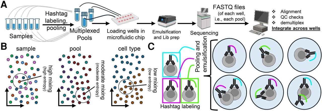
Robust data collection, in which biological effects are well preserved but technical noise is minimized, is central to the generation of rigorous data that drives genomics research. Although there is an increasing reliance of the use of single-cell RNA-seq (scRNA-seq) data to power contemporary hypothesis generation, both experiment design and data analysis in this area require extra caution. These methodologies require significant amplification of transcripts in each cell during the preparation of libraries, which can amplify well-to-well variability stemming from technical rather than biological reasons. It is widely accepted that sample multiplexing, whereby cells from different groups in the same experiment are individually barcoded and then combined in the same well, is a major innovation designed to circumvent this problem (Cheng et al. 2021; Zhang et al. 2022). Several methods for multiplexing and subsequent computational demultiplexing have been proposed (Kang et al. 2018; Guo et al. 2019; Huang et al. 2019; Shin et al. 2019; Xu et al. 2019; Srivatsan et al. 2020) with hashtag-based ones (Stoeckius et al. 2018; Gaublomme et al. 2019; McGinnis et al. 2019b; Mylka et al. 2022; Brown et al. 2024; Zhu et al. 2024) becoming more common recently. In a typical hashtag-assisted workflow, which is also used in this paper, specific samples are computationally retrieved from the sequence data, based on the expected identifying hashtags (Fig. 1A). The benefit of sample multiplexing is not just in the mitigation of batch effects (see below) but also in a reduction in per-sample cost because this allows an investigator to analyze fewer cells per group in a single well rather than dedicate the maximum capacity of each well to just one group (Pankaew et al. 2022).
A cartoon overview of a typical single-cell experiment, estimation of batch effects and hashtag labeling. (A) Overview of an in-house, single-day, scRNA-seq experiment in a laboratory. Samples are labeled with hashtags and combined for multiplexing. Each multiplexed pool is loaded into separate wells on a microfluidic plate (e.g., 10x Genomics chips) for droplet capture and reaction. The libraries are sequenced, and reads from each well (i.e., the pool) are separated based on the indexes they receive during library preparation. FASTQ files are then taken through the computational pipelines of alignment, quality control, demultiplexing, etc. Finally, the data from all the wells in that experiment are integrated to mitigate batch effects. (B) In scRNA-seq data analysis pipelines, the cells are projected in lower-dimensional spaces (e.g., principal component space or further corrected integrated spaces) based on their transcriptome. Generally, 30–50 dimensions are used, but in the cartoon shown here, a two-dimensional space is depicted for illustration. Each cell can have different attributes, also known as metadata, as depicted by different colors here within each subplot: sample (left), pool (middle), cell type (right), etc. In the absence of batch effects, similar cells from different pools and samples will be well mixed in this space, because they will not have batch-related differences in their gene expression other than biologically relevant differences. The lower the batch effects, the higher the diversity of a cell's neighborhood and the larger the entropy of that cell for those particular metadata. Typically, cell-type metadata have low mixing compared with those of samples and pools, because cells of the same type are expected to remain together in the reduction space. (C) A cartoon of emulsion droplets with hashtag-labeled cells. Generally, they are individual cells with one predominant hashtag (top circles). In some cases, more than one cell can be in a droplet (left bottom circle). Or one cell may be labeled by more than one hashtag owing to ambient hashtag antibodies after pooling (middle bottom). Alternatively, the emulsification process might capture free antibodies in the medium (right bottom). This figure is created with BioRender (https://www.biorender.com).
“Batch effects,” as we use it in this paper, is an umbrella term encompassing the variations originating from the differences in protocols, handling personnel, equipment, reagents, conditions and duration of the experiments and subsequent sample storage, library preparation, and sequencing instruments (Tran et al. 2020; Lütge et al. 2021; Ryu et al. 2023)—but are not “biological” in origin. Batch effects can be global, affecting all cell types (e.g., library prep steps), or can be local, influencing specific cell types or perhaps specific genes (e.g., storage duration/conditions affecting seq data) (Courel et al. 2019). Currently, there is no consensus on the methods of measuring batch effects in scRNA-seq data or on how much batch variation is “allowed” in different types of data sets when measured by applying the latter disparate methods (Lütge et al. 2021; Luecken et al. 2022). Patently, considerations of batch effects are also important for meta-analysis of scRNA-seq data sets (activities commonly referred to as “atlasing”), those that originate from different laboratories, following different experimental protocols, and are generated through different microfluidic and sequencing technologies (Ming et al. 2022; Ryu et al. 2023; Zhang and Zhang 2024; Hrovatin et al. 2025).
To contextualize the confounding factors in each multiplexing design, it is important to accurately measure the batch effects in each case. One of the widely used metrics in the literature to measure batch effects is entropy (in this paper “entropy” always indicates “normalized Shannon entropy”; Methods) (Fig. 1B; Chazarra-Gil et al. 2021; Lütge et al. 2021). This metric, borrowed from information theory, is intuitively straightforward for the measurement of batch effects in single-cell data. Individual cells are projected in lower-dimensional space based on their transcriptome (or chromatin accessibility), and biologically similar cells from different “batches” should be randomly mixed in the neighborhood of a given cell in the latter space. For each cell, its entropy is the measurement of the numeric mixing of its neighboring cells from different “batches” (Fig. 1B, see figure's legend).
Hashtag multiplexing itself has the potential to introduce noise (Fig. 1C). Apart from the trapping of multiple hashtagged cells or ambiently available hashtag antibodies within each sequencing reaction droplet (Fig. 1C, see figure's legend) during the microfluidic emulsification process, there is a possibility of hashtags “jumping” between cells after pooling because the hashtags are against the same antigens (Li et al. 2024; Zhu et al. 2024). All reads from some of these latter droplets (Fig. 1C, bottom circles) will be discarded during computational demultiplexing and from downstream analyses. Thus, all multiplexing processes are inherently lossy to different extents (Stoeckius et al. 2018; Shin et al. 2019). It is generally argued that such potential loss of reads/cells owing to multiplexing is the nonnegotiable collateral for batch-effect mitigation. However, to our knowledge, a systematic evaluation of the batch effects and costs of different experimental design strategies, including the use of hashtag-multiplexing, has not yet been performed.
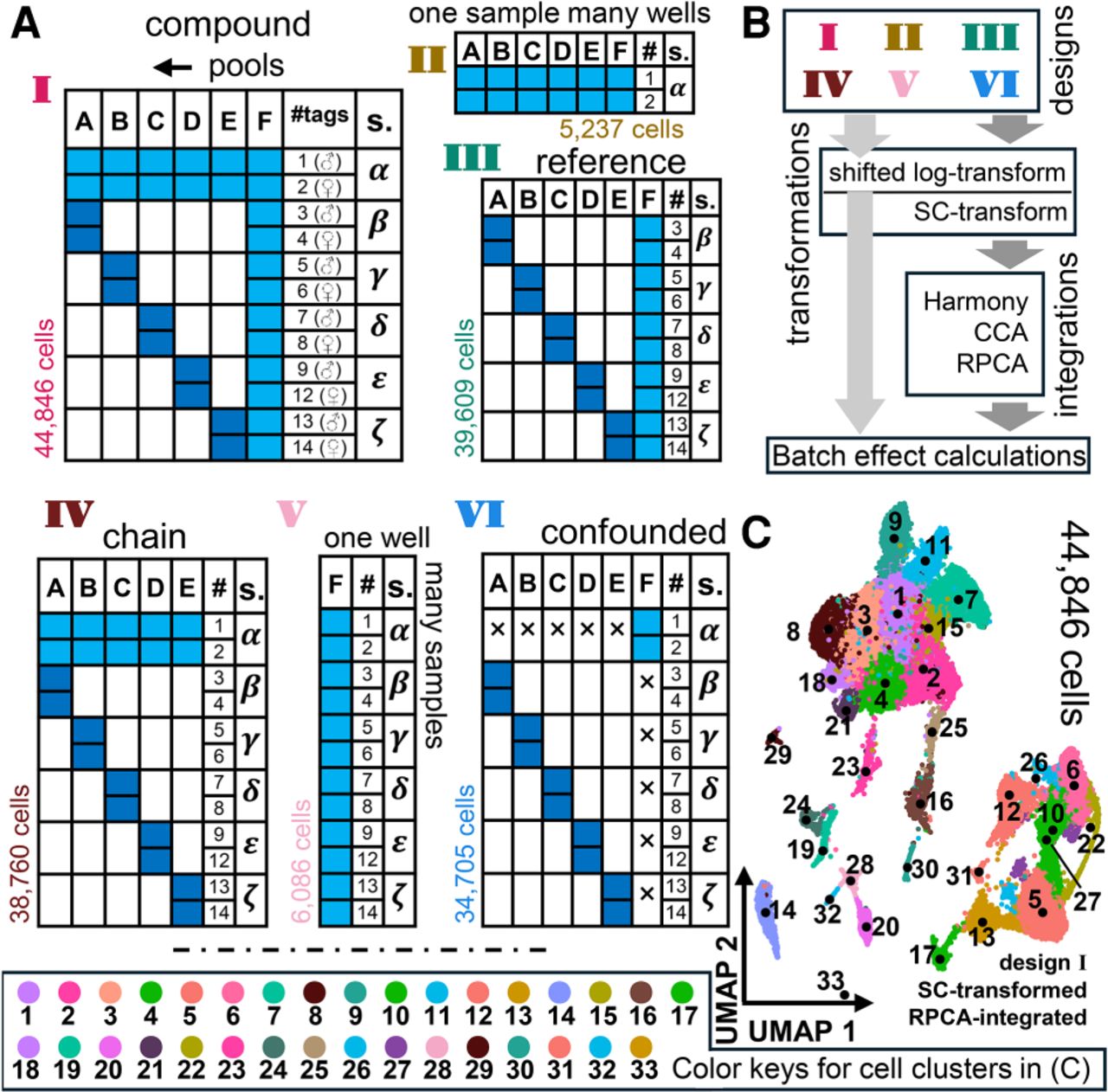
In this paper, we evaluate batch effects inherent in scRNA-seq pipelines by designing a single compound experiment (Fig. 2A, I). From this compound experiment, we then extract four major single-cell experimental design strategies, namely, single pool, reference, chain, and confounded (Fig. 2A, II–VI), thereby ensuring that each design is being compared without having been processed with additional variations in wet-laboratory execution. Using this approach, we quantify batch effects (using entropy as the metric) as well as the cost imposed owing to the loss of cell recovery at the stage of hashtag demultiplexing, resulting from each experiment design strategy. As a result, our analysis allows a user to concurrently evaluate the risk of batch effects and the cost inflicted by losing cell recovery from any particular choice of experiment design and suggests considerations that balance both criteria.
Different designs of experimental data and succeeding analytical recipes. (A) Different designs of data that are considered for batch-effect calculations. Columns in each chart indicate wells (i.e., pools A–F); rows indicate samples (α–ζ, and hashtags 1–9, 12–14). Each design is indicated by colored boxes on each chart. The lighter blue boxes indicate four times higher loading of cells compared with those in navy blue. The number of cells in each design and the design numbers in Roman numerals are shown in colors matching those used in the next figures. Design I illustrates the compound format used in the entire experiment. Descriptions of designs II to VI are given in the text. (B) A schematic of the analytical pipeline of taking the designs through the transformations, integrations, and batch-effect calculations. Light gray block arrows indicate all designs; dark gray block arrows, all except design V. For the details of the tools used under each step, see text. Each instance of the pipeline consists of one item from each of the three boxes in the diagram, namely, designs, transformations, and integrations. The latter is skipped for the “unintegrated” processing (light gray arrow) as indicated in subsequent figures. (C) UMAP on RPCA integration on the entire data, namely, design I, post SC-transformation. Contrasting colors are used for the adjacent clusters for the ease of visualization. The keys to the colors of the cell clusters are indicated in the box at the bottom. The convention of color keys used in this specific UMAP is not followed in any other figure panel in this paper. The median representative points of each cluster are indicated with a black dot along with immediately adjacent annotations of the respective cluster IDs. The annotated medians are to be used in conjunction with the color keys at the bottom; similar colors may have been used for two clusters in a limited number of instances, such as 1 and 18, 4 and 10, etc., owing to the restricted availability of adequately contrasting colors. These instances of using the same color for two clusters are carefully chosen such that the specific pair of clusters is far from each other in the projection space. Clusters 26 and 27 are split in the UMAP (splitting of cell clusters owing to projection is not unusual and is observed routinely). Thus, for instance, the median of cluster 27 lies in the middle of two split populations. The medians are plotted for the ease of visualization only; they are not related to the clustering algorithm used (see Methods).
Results
An integrated single-cell experiment for identifying batch effects across different designs
The experimental data used in this analysis are derived from an ongoing analysis of mouse splenocytes treated in vivo with five different variations of plasmid-encoded cytokines of the interleukin 12 (IL12) family compared with a control plasmid. Because the biology of these cytokine groups themselves is not relevant for our current analyses, we refer to this as a pool of six different samples—α, β, γ, δ, ε, and ζ—in different combinations in six different wells—A, B, C, D, E, and F (Fig. 2A, I). Sample α is the baseline or control group, and the rest of the samples are experimental groups. All pools received sample α. Pools A to E received one more sample other than α but no other sample. Pool F received all samples. Each sample was a 50:50 mix of female and male mice, and each received unique hashtags before pooling.
After sequencing, alignment, quality checks, and demultiplexing (Methods) (Fig. 1A), we extracted six designs from the experiment for further numeric assessments. The whole experiment, which we called a “compound” design, is denoted as design I. We then selected all α samples from all wells and denoted this as design II (Fig. 2A, II). Next, we removed the α samples from design I to form a “reference” design of single-cell experiments, which is denoted as design III (Fig. 2A, III) (Song et al. 2020). We define a “reference design” as one in which one pool contains all samples to serve as a “reference,” and the rest of the pools have only some of the samples. In design IV, we removed pool F, hence this became the “chain” design, in which pools share certain samples (sample α in this case) but there is no “reference” pool (Fig. 2A, IV). We kept only pool F with all samples as design V (Fig. 2A, V). Lastly, in design VI, we removed all of sample α from wells A–E and samples β–ζ from well F (Fig. 2A, VI). This design is also called the “confounded” design, in which no pool shares samples and there is no reference pool. Intuitively, one might expect for design I to have the least technical variation between the samples and for design VI to be the noisiest.
We then processed the data in each design through three computational steps: transformation, integration across pools, and measurement of batch effects (Fig. 2B). For the analysis of scRNA-seq data sets, currently there are 22 different methods for transformation (Ahlmann-Eltze and Huber 2023), 21 unique methods for integration (can be applied with or without highly variable gene [HVG] selection and scaling as the preprocessing step) (Tran et al. 2020; Chazarra-Gil et al. 2021; Luecken et al. 2022), and eight different ways of evaluating batch effects (Lütge et al. 2021). Although there are several tool benchmarks available for these different steps (Sonrel et al. 2023), evaluation of the best pipeline, which is a combination of three steps, would be computationally prohibitive (22 transformations × 4 preprocessing options × 21 integrations × 6 designs × 8 batch-effect calculations). Instead, we identified single-cell benchmarks based on the literature and used consensus tools for these different steps (tools that performed well across different benchmarks, diverse data sets, and conditions). For transformation, we chose the shifted log transform and SC-transform (Hafemeister and Satija 2019; Ahlmann-Eltze and Huber 2023). For integration methods, benchmarks are unclear (Tran et al. 2020; Chazarra-Gil et al. 2021; Luecken et al. 2022), but we use harmony (Korsunsky et al. 2019), CCA (Stuart et al. 2019), and RPCA (Hao et al. 2024) “anchor” integrations. Of course, there are other tools with similar potential performance capabilities that are not considered here in the interest of time and effort (Methods) (Supplemental Figs. S1, S2A,B; Haghverdi et al. 2018; Lin et al. 2019; Song et al. 2020). We used a shifted-log-transformed (“log-transformed” from here onward) but unintegrated version for all designs (see Methods) (Fig. 2B, light gray arrow on the left). Design V was not included in the integration pipelines (Fig. 2B, dark gray arrows on the right) because this involves just one pool (i.e., did not require an integration step; see Methods). The numeric projections for qualitative visualization (i.e., UMAPs) of each design, going through each combination of integration pipeline, have been documented (Supplemental Figs. S1, S2). We show one of the 31 scenarios (2 transformations × 3 integrations × 5 designs + design V) here: the SC-transformed, RPCA-integrated design I projected as a UMAP, consisting of 33 cell clusters (Fig. 2C).
Evaluation of batch effects across experimental designs and data-analytical pipelines
Conventionally, different pools/wells are called batches (i.e., the RNA-seq library in each case is prepared separately in different tubes or wells). However, the pooled samples may also have batch effects apart from their expected biological effect–driven variations owing to possible differences in sample preparation steps. We intended to quantify the influence of integration methods on these different types of batch effects (for the details of integration pipelines and batch-effect measurement, see Methods) (Stuart et al. 2019; Ryu et al. 2023; Wang et al. 2024). We, therefore, measured both types of batch effects (i.e., pool and sample) in all designs and compared the entropy distributions of integrated and unintegrated outputs for the designs. These were then compared with the cell-type entropies as a control group, because the latter are biologically expected to remain low in contrast with those of the pools and samples (Methods) (Fig. 1B).
The design with the highest median pool entropy, that is, least batch effect (for pool), before integration was design II (median entropy = 0.842, that of design I = 0.772, design IV = 0.767) (Fig. 3A, top). In this context, higher entropy indicates better mixing of cells from different pools in the lower-dimensional space. The least pool “batch” effect in design II is consistent with previous analysis of nuclear hashing experiments reporting that hashed nuclei representing the same sample generally show negligible differences when they are processed in different wells (Gaublomme et al. 2019). We further validated this by evaluating the differentially expressed transcripts between sample α from pool A versus the rest of the pools B–F (Fig. 3B, two plots on the left; Supplemental Fig. S3A). We observed very minor (one disparate upregulated DEG in three comparisons; 11 and 13 DEGs in the rest of the two comparisons, respectively), mostly nonoverlapping (three common genes in comparisons with more than one DEG) gene expression differences across five DEG comparisons, and none were significantly enriched for any biological function (Fisher's exact test, cutoff P-value = 0.01). As a positive control, we compared the samples α versus β in pool A and in pool F from designs IV and V, respectively (Fig. 3B, plot on the right; Supplemental Fig. S3B). For these between-sample comparisons, in contrast with the within-sample comparisons (Supplemental Fig. S3A), we observed that 55 and 97 genes were upregulated (Fig. 3B, plot on the right; Supplemental Fig. S3B), respectively, among which 47 were common. We used the median of the pool entropy for design II as a threshold (Fig. 3A, top panel, dashed line) and checked the percentage of cells in other designs that are above it. Although ∼25%–30% of cells in designs I, III, and IV were above the threshold, design VI (the confounded design) elicited a mere 11% of cells above the latter.
Estimation of batch effects in different designs before and after data integration. (A) Entropies of each cell in different designs are measured, and the distributions of the entropies are presented as violin plots. Entropies of pools (top), samples (middle), and cell clusters (i.e., cell types; bottom) are shown. For design V and design II, pool and sample entropies, respectively, are not shown (see text; Methods) (see Fig. 2A). The percentages on the x-axis are percentages of cells above the threshold (dashed gray line) that were chosen as the median of the pool entropy for design II. (Unint) Unintegrated; (LT) log-transformed. (B) Representative volcano plots to compare gene expression in cells from the same sample but different wells (left) and the same well but different samples (right). All plots are shown in Supplemental Figure S3. Dashed horizontal lines indicate P = 0.01. The colors in the volcano plots are for the ease of visualization and are not linked to the color schemes in any other figures. (C) Same as A but looking at the mixing in SC-transformed RPCA (see text) integrated reduced space. Design V is excluded in this representation because this design has only one well, hence cannot be integrated. (SCT) SC-transformed. (D) Percentage of cells above the pool (left) and sample (right) entropy thresholds obtained with three different integration strategies (Harmony, CCA, RPCA; see text) for designs I, III, IV, and VI. The dashed line represents 50%.
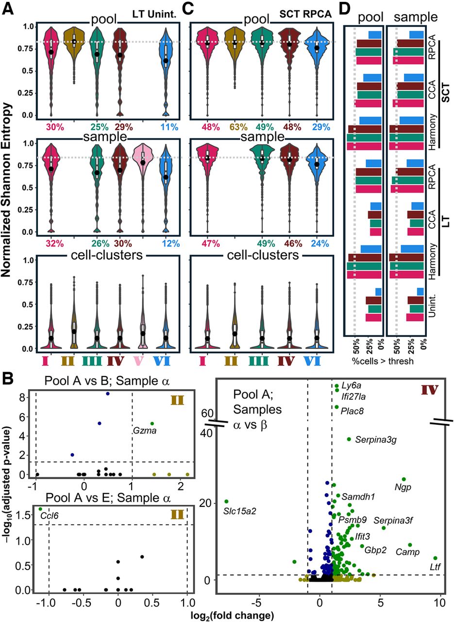
In the sample entropy calculations, the unintegrated design V showed the highest performance (median entropy = 0.839, that of design I = 0.791, design IV = 0.771) (Fig. 3A, middle panel), as expected, because this is a reference pool in which all the samples are processed together in the same well. We therefore used the median of the sample entropy distribution of design V as the sample entropy threshold (Fig. 3A, middle panel, dashed line) to check the sample “batch” effects in the other designs. The rationale here is that any pipeline of transformation/design/integration that would yield ≥50% cells above the latter entropy threshold is performing as well as the “biological” sample mixing observed in the reference pool (i.e., pool F, design V). Recall that pool F contains all samples of our experiment processed by identical reagents/instruments/experimentalist; hence, we expect minimal sample “batch” variation and no pool “batch” variation at all (i.e., cells are from just one well, F). Hence, the median entropy of cells in this pool can be a useful global threshold for the acceptable extent of sample “batch” correction in similar biological samples. Using this criterion, we find that in designs I, III, and IV, 26%–32% of the cells were above the entropy threshold, supporting the consensus that semi-independent processing of the pooled samples in different wells may compound the limited sample “batch” variations. Again, design VI was the worst performer, with only 12% of the cells above the threshold. The cell-cluster entropy distributions showed much lower medians (range of medians of entropy for designs I–VI: 0.077–0.191) (Fig. 3A, bottom panel), as we would expect.
Calculating the entropy distributions postintegration (Fig. 3C; Supplemental Fig. S4) using a representative transformation/integration approach (SC-transform, RPCA integration), we found that designs I, III, and IV consistently reached ∼50% of cells above the respective thresholds of pool and sample entropy distributions, conforming to the expected reduction in batch effects owing to integration. However, the integration process could not recover the batch effects of design VI for either sample or pool. The performances of all transformation/integration scenarios are summarized in Figure 3D. All integration methods in both transformations brought the desired 50% cells (Fig. 3D, dashed line) above the entropy threshold (because the thresholds were the medians from the respective contexts), except for the log-transformed CCA. For harmony and RPCA, the SC-transformation did not provide added benefits over the log transformation. Notably, it has been shown before in a previous benchmark that the latter performs “surprisingly well” (Ahlmann-Eltze and Huber 2023). To conclude, no integration method could fully recover the batch effects in design VI; in other words, designs III and IV always performed better than VI irrespective of the subsequent computational pipeline, emphasizing that some designs are always better than others.
Efficacy of the hashtag-assisted multiplexing and demultiplexing processes
We then evaluated the labeling efficacies of the hashtags used. Droplet doublets (Fig. 1C, bottom left circle) often tend to have higher counts and features than the singlets (Luecken and Theis 2019; Germain et al. 2022). We used the HTOdemux function of the “Seurat” package to perform the demultiplexing (Howitt et al. 2023; Li et al. 2024; Sayed et al. 2025) and found that the distributions of the doublets are largely overlapping with those of singlets; that is, ∼50% counts or features in doublets are below the third quartile threshold in singlets in the distributions of counts and features from the pools A–F (Supplemental Fig. S5A,B). This suggests that a large percentage of hashtag doublets (Fig. 1C, bottom, middle, and right circles) are indeed droplet singlets (Li et al. 2024; Zhu et al. 2024). A fraction of these could also arise from droplet doublets, resulting in hashtag doublets, as reported originally (Stoeckius et al. 2018).
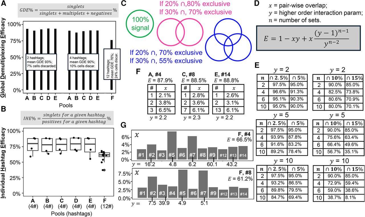
We reasoned that a quick way to measure the global efficacy of hashtags in a pool would be to calculate the percentage of total number of singlets against the total number of cells, within that pool (global demultiplexing efficacy [GDE]) (Fig. 4A). The closer this metric is to 100%, the more successful the entire pooling and demultiplexing would be. For scenarios using two and four hashtags (pools A–E), the GDE was 93% and 90%, respectively. But for pool F, it falls abruptly to 76%, indicating that with a higher number of hashtags more cells are likely lost as nonsinglets. To understand the relationship between use of higher number of hashtags and the number of cells lost as multiplets in a given pool, we calculated individual hashtag efficacy (IHE), which is the percentage of singlets for a given hashtag against the total number of cells that are positive for that hashtag (Fig. 4B). Several demultiplexing software, including HTOdemux, declare a lower threshold (i.e., a background level) of reads (of the specific hashtag oligomer sequence) to designate a cell to be “positive” for that hashtag (Xin et al. 2020; Howitt et al. 2023; Klein 2023). Thus, a cell can be “positive” for more than one hashtag (i.e., a doublet/multiplet); ergo, singlets are the cells that are “positive” for only one hashtag. In other words, for an individual hashtag, the singlets are a subset of the positives; accordingly, IHE is the ratio of the former to the latter. IHE for the hashtags in pools A–E showed a median of ∼80%. Again, in pool F, there was a sharp fall of the IHE, although the same hashtags as used in A–E were used in F, but all of them together. This means that the efficacy of the hashtags was dependent not only on the hashtags themselves but also on how many of them are being used simultaneously.
Evaluation of the performance of hashtags in demultiplexing: (A) Evaluation of global demultiplexing efficacy (GDE) in each pool. Bar diagram showing percentage of hashtag singlets within all cells in a well. The first five bars are the calculations of GDEs of wells A–E, combining two hashtags within a sample as one. The approximated mean GDE is noted on the boxes covering the lower parts of the bars. (B) Evaluation of individual hashtag efficacies (IHE) for each hashtag used in each pool shown as dot plots accompanied by overlaid box plots. Pools and the number of hashtags (in brackets) used in them are marked on the x-axis. The hash (#) signs are abbreviations for “hashtag.” For A and B, the expressions of GDE and IHE, respectively, are noted in the gray boxes at the top. (C) Cartoon Venn diagrams to illustrate the relations between overlaps and the availability of exclusive parts of intersecting sets. (D) A closed-form expression to calculate exclusive parts of sets (E), given that we know x, y, and n (see text) (Supplemental Text S1). (E) Charts showing calculations of E, for the given value of y and x (shown at the top of the charts). The different values of x are at the top row, preceded by a ∩ (intersection) sign, and n is the first column in the charts. (F,G) Estimation of x and y in single-cell data. Three charts are for the pools with four hashtags; the first columns indicate the specific hashtag for which the overlap is calculated, and the second columns are the estimated values of x (F). Two bar plots at the bottom are for pool F, namely, 12 hashtags (G). The title above the charts/bar plots, such as “F, #4,” indicates that x and y are estimated for hashtag 4 in well F. Below that, the percentage of exclusive signals, namely, singlets for that hashtag, is noted. The bars or the second columns of the charts are the values of x, as estimated directly from data (see Methods). Numeric estimates of y are noted immediately below the bars or the chart entries (i.e., the corresponding x values).
A theoretical framework for analyzing the effects of hashtag multiplexing
Intrigued by the sharp fall of GDE and IHE in pool F, we built a theoretical framework to better understand the origins of hashtag noise. We consider all cells positive for a given hashtag to be equivalent to a mathematical set. Because hashtag signals interfere with each other, potentially through different mechanisms (Fig. 1C), these sets of positive signals can potentially overlap with each other (Fig. 4C, illustrative Venn diagrams). As the number of such sets (i.e., number of hashtags) increases, the area of overlap is expected to increase, with a parallel decrease in the exclusive parts of each set, unless all higher-order intersections (common overlap regions of multiple sets) tend to accumulate on the same cells. We derived a closed-form expression to calculate the exclusive regions (E) of a set in a universe of multiple interacting sets (Fig. 4D, gray box; Supplemental Text S1) based on the simplifying assumption that the intersections are symmetric; that is, all hashtags show similar overlaps with each other. This closed-form expression depends on three variables: pairwise overlap x, higher-order interaction parameter y, and number of sets (i.e., hashtags) n (Methods) (Supplemental Text S1). Note that y ≥ 1, and higher values of y mean that the positive signals for multiple hashtags are increasingly not showing up in the same cells. Ergo, higher values of y will eliminate exclusive signals, as indicated by our closed-form expression. Calculating E with realistic values (see below) of x, y, and n (Fig. 4E) with increasing x, y, and n, confirms that the exclusive signal decreased rapidly. Thus our theoretical framework, which is a minimalistic representation of the hashtag multiplexing and demultiplexing process, indicates that demultiplexing efficacy will increase (i.e., the abundance of singlets will increase) with decrease in the number of hashtags in an experiment (lower n), with decrease in the tendency of the hashtags to participate in binary overlaps, namely, to generate doublets (lower x), and, somewhat counterintuitively, with increase in their collective propensity to generate multiplets (higher 1/y).
Next, we estimated x and y of the hashtags in our pools (Fig. 4F,G) by randomly selecting hashtags and calculating x as the percentage of cells that are positive for both, specifically the given hashtag and the rest of the hashtags in the pool. Unfortunately, our closed-form expression cannot be explicitly solved for y when n > 3. Because our n is four or higher, we used numeric (bisection) methods to estimate y from known x, n, and E. The estimates of y were always lower in pools with n = 4 (Fig. 4F) compared with the estimates of y in pool F (Fig. 4G). Our model fitting confirms the intuitive understanding that with increasing the number of hashtags in a pool, the fraction of singlets keeps decreasing because of the nonoverlapping lower-order (binary) intersections, that is, rapidly diminishing higher-order intersections.
A statistical model of hashtag multiplexing
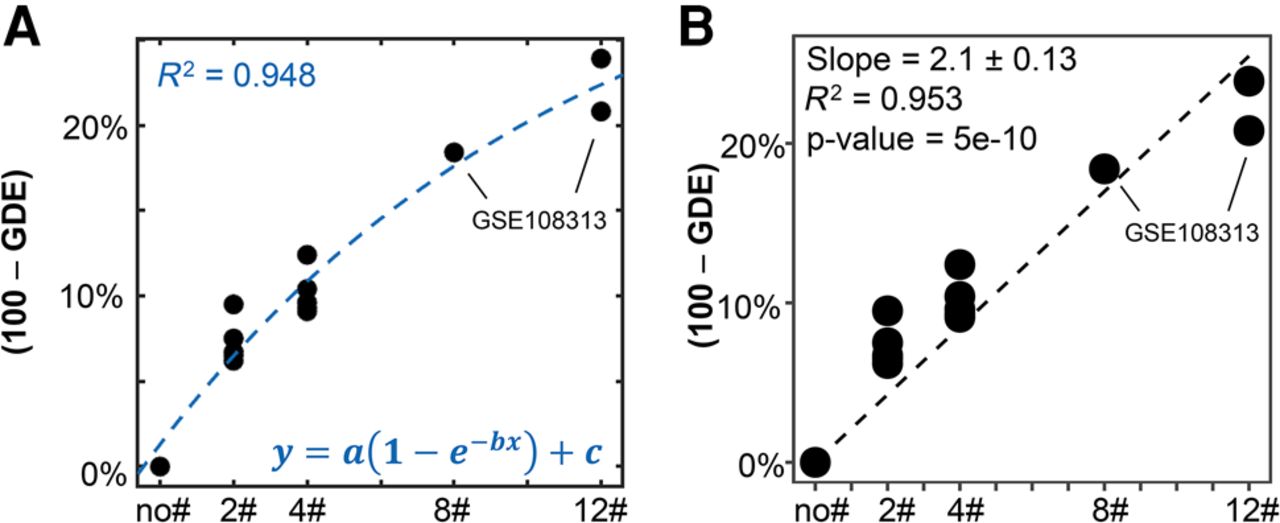
To compare the results obtained with our data to previously reported external data sets, we used a published (Stoeckius et al. 2018) data set. We fitted the number of hashtags used in a pool to the percentage gap between GDE and 100 in the respective pool using nonlinear regression models first, because visual inspection of the data indicated a minor tendency toward a saturation effect (Fig. 5A, dots). The exponential decay model (R2= 0.948) (Fig. 5A) performed better than a logarithmic model fitting (R2= 0.882). Next, for ease of interpretation, we attempted a linear regression on the same data (Fig. 5B). Indeed, we observed a highly significant positive slope in this analysis. The quality of the fit (i.e., the R2) was similar to that of the nonlinear fit. This observation again directly supported the interpretation from our theoretical framework: With an increasing number of hashtags (n), the demultiplexing efficacy decreases. The linear regression analysis further indicated that for every hashtag added to a pool, the percentage of cells lost will double (e.g., 14% cell loss for seven hashtags). Note that currently, it is possible to superload wells with 24 hashtags (antibody based).
Statistical modeling of hashtag demultiplexing: (A) The difference between GDE and 100 (as percentages) is plotted on y-axis for different pools and the number of hashtags in respective pools in the x-axis, from the current data set and another external data set (GSE108313). Nonlinear regression analysis was carried out using the exponential decay model (the increasing form, equation at the bottom) on the data set. The blue dashed line represents the best fit nonlinear model. R2 of nonlinear regression is mentioned at the left top. The estimated values of the parameters a, b, and c with 95% CI are as follows: a = 32.6 (14.53, 50.68), b = 0.08661 (− 0.001616, 0.1748), c = 1.3 (− 1.477, 4.077). (B) Linear regression on the same data as in A. The dashed line is the best-fit linear model. Slope, P-value, and R2 of linear regression on the data points are recorded at the left top.
Discussion
Hashtag contamination and capture of cells in droplets during emulsification are stochastic molecular processes. Hence, the overlaps of such interactions are expected to get compartmentalized, resulting in the loss of exclusive signals with an increase in the number of samples. Hence, the increased estimates of the parameter y in pool F (Fig. 4G), that is, the parameter whose inverse represents the higher-order interaction between multiple hashtag sets, are perhaps expected from a chemical kinetic perspective, too.
Here we carried out a single-cell experiment and generated six different data designs for the evaluation of postintegration batch-effect-mitigation, reflecting different experimental designs, and for the quantification of the extent of cell loss owing to hashtag-assisted superloading. We carefully controlled well-known factors contributing to batch effects: reagents, instruments, same-day execution, and, of course, the same protocol for sample processing, library preparation, and sequencing. Although our paper is based on a CITE-seq experiment, we speculate that our conclusions should be generally applicable to any other droplet-based single-cell sequencing technique that involves sample multiplexing through hashtagging (Gaublomme et al. 2019; McGinnis et al. 2019b; Boughter et al. 2025).
The version of the “chain” design we used here is one possible version of the chain design, which we call a “baseline” chain design. There can be another “diagonal” chain design that would involve α, β, and γ in pool A; β, γ, and ε in pool B; γ, ε, and ζ in pool C, and so on. Originally, the latter was discussed in the theoretical treatment of batch correction methods of data sets with disparate cell types by Song et al. (2020). However, we were influenced by the study that reported more stable downstream analysis results achieved through the addition of small fractions of spiked-in baseline cells (Marquina-Sanchez et al. 2020). Hence, we followed the “baseline” chain design here. An additional advantage of this approach was being able to calculate the pool entropy threshold. We anticipate that the baseline chain design will also open the possibility of using postintegration, design-aware statistical finetuning for biological signal preservation across batches (Zhang et al. 2025).
In typical hashtag-based multiplexing experiments, a small population of cells can often be unlabeled (remain hashtag negative) owing to technical limitations with antibody binding or antigen expression. In our analysis, we model the cells with positive signals only (Fig. 4C–E), but it should be noted that in different experimental conditions in which the proportion of hashtag-negative cells is much higher than ours or previously published hashtag benchmark data sets (e.g., GSE108313), their contribution may need to be controlled for.
We proposed here a within-experiment threshold of entropy to assist in batch correction. If the majority of the cells in the integrated data are above this threshold, there is a possibility that the data set is overintegrated and thus leads to the removal of biological signals. We would suggest investigators take appropriate precautions to prevent such scenarios, depending on the experimental and biological context that they are investigating.
Our study has limitations. The first limitation of our study is that we evaluate only a very small number of combinations of the methods of integration and transformations here. However, most of the ones we tried worked satisfactorily, in other words, the desired percentage of cells reached or crossed predefined entropy thresholds, and hence, we think that if a batch-effect threshold is known, the choice of the integration method should be up to the investigator, in particular because parameters in most integration methods can be further tuned to get to the threshold. Because of cost considerations, we could not include compound design experiments with pools with intermediate (4 < n < 12) or very high (12 < n < 24) numbers of hashtags, though using an external data set helped us partially address such gaps (Fig. 5). Notably, it is possible that there is a saturation effect in cell loss for very high numbers of hashtags, that is, n > 12 (to inspect the trend of the data for n ≤ 12, see Fig. 5A), which we have not studied here. We expect that future efforts will address this gap. However, within the range of number of hashtags that we investigate here, there is a robust linear relationship between cell loss and n (Fig. 5B). We also note that we have not tested for the scenario of combinatorial hashtag indexing here (McFarland et al. 2020; Fang et al. 2021; Hwang et al. 2021). Combinatorial hashtagging or using SNPs alongside hashtags for demultiplexing are specialized, powerful methods used much less frequently for routine single-cell experiments, in our experience. Nevertheless, it will be interesting to contextualize our theoretical framework with combinatorial hashtagging data sets. The application of doublet detection and removal techniques can further contribute to higher demultiplexing efficacy (McGinnis et al. 2019a; Germain et al. 2022). However, the benefits of prior doublet detection in demultiplexing are not well understood. Further, ambient RNA contamination across the microfluidic droplets might interfere with the quality of data integration and subsequent clustering (Yang et al. 2020). How computational decontamination algorithms influence experimental designs and, subsequently, the performance of the batch correction methods needs more attention in future work. We also note that a source of variation in our data set stems from differences in individual samples, for instance, the specific cytokine made in the sample α versus β. Overall, this biological effect was minimal in our analysis, as we did not observe significant global transcriptional shifts from any particular treatment (Supplemental Fig. S2, sample mixing). However, this would be a factor to consider in a more rigorous benchmarking experiment. Another limitation is that moderated experimental design, which we propose as a measure for controlling batch effects and cell loss, of course, is not applicable for the literature-based atlasing activities. However, if a laboratory or a consortium is planning experiments to build a new atlas through fresh experiments, the moderated designs we discussed here can be quite useful to maximize cell yield and yet gracefully integrate the data.
Here we carried out a controlled comparison of whether and how different single-cell experimental designs can impact both batch-effect mitigation and cell recovery. To that end, we performed one overall experiment (Fig. 2A, I) and then extracted multiple designs from the data to evaluate the efficacy of the different designs at the data analytical steps of integration and demultiplexing. We reasoned that the factors influencing independent experiments, such as antibody concentrations, pipetting errors, differences in cell adhesion to each tube, antibody binding, physical aggregation of antibodies, etc., can influence both batch effect and cell recovery through further interference with the downstream analytical steps that we are focusing on here (i.e., integration and demultiplexing). Extracting the designs from one overall experiment helped us decouple experimental variations from the analytical performance metrics. Nevertheless, the next step in this inquiry would be to combine an analysis of more “real-world” experimental designs and interrogate how biological noise from disparate experiments can further modify batch effects and cell loss.
We conclude here that reference or chain multiplexing designs can reduce the number of hashtags used, and batch effects can be satisfactorily mitigated through integration of the pools. Thus, cell loss through superloading and batch effects across pools can be balanced through refining experimental design. Moreover, in the “reference” design (design III), a threshold is possible to know for the extent of biological mixing in the samples, and different integration methods can be attempted or integration parameters can be finetuned until such level of mixing is not achieved while integrating across pools. Although a compound design (design I) can provide acceptable thresholds of batch effects for both samples and pools, which can be subsequently used for optimization of the integration, the more convenient reference designs can be picked because they perform similarly well for data integration. A confounded multiplexing design, although more convenient to carry out for serially incoming samples, will be more challenging regarding correction of its batch effects. We provide here an initial rubric to choose experimental designs that are appropriate for the demands of each experiment: For example, for patient samples or clinical isolates, higher multiplexing should be preferred, whereas for investigations of rare cell types or for atlas building experiments, lower multiplexing will be the goal to maximize the number of retrieved cells; both of these extremes of biological scenarios and the intermediates thereof, however, can remain within the brackets of reference or chain designs that we discussed here.
Methods
Data generation for use in analysis
The biological experiment involved the injection of expression constructs of the IL12 protein family as plasmids in mice using hydrodynamic injection. Different versions of plasmids expressing IL-12P40 or variations therein were used (Abdi et al. 2014; Abdi and Singh 2015) but are not discussed here because the ensuing phenotypes are not studied here. The plasmid injections were performed in mice, and typically the plasmids transform cells in the liver. We then analyzed cells isolated from the spleen (Supplemental Table S1). As such, these manipulations caused minimal changes in gene expression in splenocytes. Notably, we carefully controlled well-known factors contributing to batch effects in our experiment: reagents, instruments, same-day execution, and the same protocol for sample processing, library preparation, and sequencing. The sample preparation steps were carried out by an individual experimentalist.
Sequencing and data extraction
The pooled libraries were sequenced in the Illumina NovaSeq platform (Psomagen) and the base call (BCL) files demultiplexed with mkfastq function of CellRanger (10x Genomics) to generate FASTQ files containing the reads of different pools.
Alignment, data cleanup, and processing
Both transcript and surface reads from each pool (i.e., index FASTQ files) were aligned with the count function from CellRanger in default settings. The filtered barcode matrices (the output from CellRanger) were further analyzed with the Seurat (v5.3.0) toolkit in R (v4.5.0) (R Core Team 2025). Six pools (A–F) were cleaned (cells with count < 20,000, 500 < feature < 3000, mitochondrial reads < 2.5% were kept for further analysis) and demultiplexed with the default Seurat pipeline (HTOdemux function) (Supplemental Fig. S6). We removed the TCR, BCR, ribosomal, and mitochondrial genes before integration because the variability within these sequences is a confounding factor independent of the design considerations of this manuscript. After cleanup, we had a total of 44,846 cells from six pools (i.e., design I).
Integration of the data designs
For a detailed description of the data designs, see Figure 2A. We carried out the overall experiment (compound design) and then extracted different designs from the data for the evaluations of the quality of integration. We avoided carrying out separate experiments for each design because that would bring in additional batch effects for the disparate experiments, making the comparisons of postintegration batch effects between the designs less meaningful.
For all designs, the following steps were taken for the transformation and integration: After merging the data from different pools in the given design, first the counts were normalized with Seurat function NormalizeData. This function carries out a shifted logarithmic transformation (Ahlmann-Eltze and Huber 2023), which is referred to as “log transformation.” Subsequently, PCA was carried out after scaling and finding 3000 most variable features, followed by cell clustering and projection (UMAP). This is unintegrated version of the designs. Next, for all designs, except design V, the following integration recipes were run at the pool level on the latter principal component space: CCA (Stuart et al. 2019), RPCA (Hao et al. 2024), and Harmony (Korsunsky et al. 2019), utilizing the IntegrateLayer function from Seurat. Further cell clustering and projecting were carried out using each of these integrated spaces. PCA was always on the first 50 dimensions, and the resolution parameter of cluster search (Louvain method) was always 1. A similar integration pipeline was carried out next, but now on the SCtransformed data (Hafemeister and Satija 2019).
The final number of clusters varied in the different designs after processing through disparate integration pipelines (Supplemental Fig. S7A). We used these numeric cell clusters to calculate the cell-type entropies (see below). As a confidence check, we manually inspected whether each cluster had orderly representation in each condition in a given design and integration pipeline (Supplemental Fig. S7B). We summarized the variation in cell abundance across clusters and conditions by averaging the coefficient of variation (CV) along with its margin of error (Supplemental Fig. S7C). Compound, reference and chain designs showed averaged CVs well below 50%. These explorations ensured that the cell-type abundances across the different conditions were largely similar, except for the context of design VI. Finally, we conducted Kruskal–Wallis tests across conditions to test the null hypothesis that the cell-type abundances are sampled from the same distribution across conditions (Supplemental Fig. S7D). Encouragingly, this test did not lead to rejection of the null hypothesis in any instance.
Measurements of batch effects
We used normalized Shannon entropy (Chazarra-Gil et al. 2021; Lütge et al. 2021) for the characterization of batch effects. Briefly, Shannon entropy quantifies the information content in the neighborhood of each cell, following the expression below:
As mentioned in the previous section, we carried out the integration process at the pool level because that is what we define as the traditional “batch” in our experiment. However, we measured the batch effect at the sample level along with the pool level. The pool-level integration methods that we use here are in principle expected to correct sample-level variations also (as we observe in Fig. 3A,C), as long as there are shared samples, that is, “cell states,” across the pools (Stuart et al. 2019; Hao et al. 2024).
Differential expression analysis across wells
Differential expression analysis was carried out (Supplemental Fig. S3) using DESeq2 package (Love et al. 2014) in R after pseudobulking the counts at the hashtag level. The differentially expressed genes were checked for enrichment of biological functions using ShinyGO (Ge et al. 2020).
Calculations of hashtag efficacy
Hashtag demultiplexing was carried out using the HTOdemux function in Seurat with the parameters set to default. Thresholds declared by HTOdemux were used further to calculate the GDE and IHE (Fig. 4A,B). The latter thresholds were also utilized for enumerating the pair-wise overlap parameter, x (Fig. 4C,D; Supplemental Text S1). The higher-order interaction parameter, (i.e., y) was estimated using the uniroot function in R for root search within predefined boundaries. For several values of x, the estimated values of y are noted in the figure; however, it can be estimated within fixed intervals for any hashtag in any pool.
Using external data
We used one external data set (Stoeckius et al. 2018) for gathering more GDE data points in our regression analysis (Fig. 4G). This data set (obtained from the NCBI Gene Expression Omnibus [GEO; https://www.ncbi.nlm.nih.gov/geo/] under accession number GSE108313) was made available in the convenient RDS format by the authors as part of the vignette for the Seurat HTOdemux algorithm.
Data access
All raw and processed data generated in this study have been submitted to NCBI Gene Expression Omnibus (GEO; https://www.ncbi.nlm.nih.gov/geo/) under accession number GSE333171. All code and data (in H5 format) for generating the main text and supplemental figures are available in the GitHub repository (https://github.com/NevilLab/Hashbatch) and also as Supplemental Code and Supplemental Data.
Competing interest statement
The authors declare no competing interests.
Acknowledgments
This project is funded by R01AI168192 from the National Institutes of Health (National Institute of Allergy and Infectious Diseases) and HR001121S0037-AIM-FP-009 from the Biological Technologies Office, Defense Advanced Research Projects Agency (DARPA).
Author contributions: B.C. and N.J.S. conceived the study. K.G., C.B., Y.O., and E.M.H. carried out the experiment and generated the libraries. B.C. and C.T.B. processed the sequencing data. B.C., M.R., and C.T.B. carried out computational analyses. B.C., M.M.-S., and N.J.S. contributed to data interpretation. N.J.S. acquired funding. B.C. wrote the initial manuscript with N.J.S. All authors subsequently reviewed, edited, and approved the final manuscript.
Footnotes
[1] Supplementary material [Supplemental material is available for this article.]
[2] Article published online before print. Article, supplemental material, and publication date are at https://www.genome.org/cgi/doi/10.1101/gr.281624.125.
[3] Freely available online through the Genome Research Open Access option.
References
- ↵Abdi K, Singh NJ. 2015. Making many from few: IL-12p40 as a model for the combinatorial assembly of heterodimeric cytokines. Cytokine 76: 53–57. 10.1016/j.cyto.2015.07.026
- ↵Abdi K, Singh NJ, Spooner E, Kessler BM, Radaev S, Lantz L, Xiao TS, Matzinger P, Sun PD, Ploegh HL. 2014. Free IL-12p40 monomer is a polyfunctional adaptor for generating novel IL-12–like heterodimers extracellularly. J Immunol 192: 6028–6036. 10.4049/jimmunol.1400159
- ↵Ahlmann-Eltze C, Huber W. 2023. Comparison of transformations for single-cell RNA-seq data. Nat Methods 20: 665–672. 10.1038/s41592-023-01814-1
- ↵Amezquita RA, Lun AT, Becht E, Carey VJ, Carpp LN, Geistlinger L, Marini F, Rue-Albrecht K, Risso D, Soneson C, 2020. Orchestrating single-cell analysis with Bioconductor. Nat Methods 17: 137–145. 10.1038/s41592-019-0654-x
- ↵Boughter CT, Chatterjee B, Ohta Y, Gorga K, Blair C, Hill EM, Fasana Z, Adebamowo AO, Ammar F, Kosik I, 2025. CountASAP: a lightweight, easy to use python package for processing ASAPseq data. BMC Bioinformatics 26: 307. 10.1186/s12859-025-06311-0
- ↵Brown D, Anttila C, Ling L, Grave P, Baldwin T, Munnings R, Farchione A, Bryant V, Dunstone A, Biben C, 2024. A risk-reward examination of sample multiplexing reagents for single cell RNA-seq genomics. Genomics 116: 110793. 10.1016/j.ygeno.2024.110793
- ↵Chazarra-Gil R, van Dongen S, Kiselev VY, Hemberg M. 2021. Flexible comparison of batch correction methods for single-cell RNA-seq using BatchBench. Nucleic Acids Res 49: e42. 10.1093/nar/gkab004
- ↵Cheng J, Liao J, Shao X, Lu X, Fan X. 2021. Multiplexing methods for simultaneous large-scale transcriptomic profiling of samples at single-cell resolution. Adv Sci 8: 2101229. 10.1002/advs.202101229
- ↵Courel M, Clément Y, Bossevain C, Foretek D, Vidal Cruchez O, Yi Z, Bénard M, Benassy M-N, Kress M, Vindry C, 2019. GC content shapes mRNA storage and decay in human cells. eLife 8: e49708. 10.7554/eLife.49708
- ↵Cover TM. 1999. Elements of information theory. John Wiley & Sons, New York.
- ↵Fang L, Li G, Sun Z, Zhu Q, Cui H, Li Y, Zhang J, Liang W, Wei W, Hu Y, 2021. CASB: a concanavalin A-based sample barcoding strategy for single-cell sequencing. Mol Syst Biol 17: MSB202010060. 10.15252/msb.202010060
- ↵Gaublomme JT, Li B, McCabe C, Knecht A, Yang Y, Drokhlyansky E, Van Wittenberghe N, Waldman J, Dionne D, Nguyen L, 2019. Nuclei multiplexing with barcoded antibodies for single-nucleus genomics. Nat Commun 10: 2907. 10.1038/s41467-019-10756-2
- ↵Ge SX, Jung D, Yao R. 2020. ShinyGO: a graphical gene-set enrichment tool for animals and plants. Bioinformatics 36: 2628–2629. 10.1093/bioinformatics/btz931
- ↵Germain P-L, Lun A, Meixide CG, Macnair W, Robinson MD. 2022. Doublet identification in single-cell sequencing data using scDblFinder. F1000Res 10: 979. 10.12688/f1000research.73600.2
- ↵Guo C, Kong W, Kamimoto K, Rivera-Gonzalez GC, Yang X, Kirita Y, Morris SA. 2019. CellTag Indexing: genetic barcode-based sample multiplexing for single-cell genomics. Genome Biol 20: 90. 10.1186/s13059-019-1699-y
- ↵Hafemeister C, Satija R. 2019. Normalization and variance stabilization of single-cell RNA-seq data using regularized negative binomial regression. Genome Biol 20: 296. 10.1186/s13059-019-1874-1
- ↵Haghverdi L, Lun AT, Morgan MD, Marioni JC. 2018. Batch effects in single-cell RNA-sequencing data are corrected by matching mutual nearest neighbors. Nat Biotechnol 36: 421–427. 10.1038/nbt.4091
- ↵Hao Y, Stuart T, Kowalski MH, Choudhary S, Hoffman P, Hartman A, Srivastava A, Molla G, Madad S, Fernandez-Granda C, 2024. Dictionary learning for integrative, multimodal and scalable single-cell analysis. Nat Biotechnol 42: 293–304. 10.1038/s41587-023-01767-y
- ↵Howitt G, Feng Y, Tobar L, Vassiliadis D, Hickey P, Dawson MA, Ranganathan S, Shanthikumar S, Neeland M, Maksimovic J, 2023. Benchmarking single-cell hashtag oligo demultiplexing methods. NAR Genom Bioinform 5: lqad086. 10.1093/nargab/lqad086
- ↵Hrovatin K, Sikkema L, Shitov VA, Heimberg G, Shulman M, Oliver AJ, Mueller MF, Ibarra IL, Wang H, Ramírez-Suástegui C, 2025. Considerations for building and using integrated single-cell atlases. Nat Methods 22: 41–57. 10.1038/s41592-024-02532-y
- ↵Huang Y, McCarthy DJ, Stegle O. 2019. Vireo: Bayesian demultiplexing of pooled single-cell RNA-seq data without genotype reference. Genome Biol 20: 273. 10.1186/s13059-019-1865-2
- ↵Hwang B, Lee DS, Tamaki W, Sun Y, Ogorodnikov A, Hartoularos GC, Winters A, Yeung BZ, Nazor KL, Song YS, 2021. SCITO-seq: single-cell combinatorial indexed cytometry sequencing. Nat Methods 18: 903–911. 10.1038/s41592-021-01222-3
- ↵Kang HM, Subramaniam M, Targ S, Nguyen M, Maliskova L, McCarthy E, Wan E, Wong S, Byrnes L, Lanata CM, 2018. Multiplexed droplet single-cell RNA-sequencing using natural genetic variation. Nat Biotechnol 36: 89–94. 10.1038/nbt.4042
- ↵Klein H-U. 2023. demuxmix: demultiplexing oligonucleotide-barcoded single-cell RNA sequencing data with regression mixture models. Bioinformatics 39: btad481. 10.1093/bioinformatics/btad481
- ↵Korsunsky I, Millard N, Fan J, Slowikowski K, Zhang F, Wei K, Baglaenko Y, Brenner M, Loh P-R, Raychaudhuri S. 2019. Fast, sensitive and accurate integration of single-cell data with Harmony. Nat Methods 16: 1289–1296. 10.1038/s41592-019-0619-0
- ↵Li L, Sun J, Fu Y, Changrob S, McGrath JJ, Wilson PC. 2024. A hybrid demultiplexing strategy that improves performance and robustness of cell hashing. Brief Bioinformatics 25: bbae254. 10.1093/bib/bbae254
- ↵Lin Y, Ghazanfar S, Wang KY, Gagnon-Bartsch JA, Lo KK, Su X, Han Z-G, Ormerod JT, Speed TP, Yang P, 2019. scMerge leverages factor analysis, stable expression, and pseudoreplication to merge multiple single-cell RNA-seq datasets. Proc Natl Acad Sci 116: 9775–9784. 10.1073/pnas.1820006116
- ↵Love MI, Huber W, Anders S. 2014. Moderated estimation of fold change and dispersion for RNA-seq data with DESeq2. Genome Biol 15: 550. 10.1186/s13059-014-0550-8
- ↵Luecken MD, Theis FJ. 2019. Current best practices in single-cell RNA-seq analysis: a tutorial. Mol Syst Biol 15: e8746. 10.15252/msb.20188746
- ↵Luecken MD, Büttner M, Chaichoompu K, Danese A, Interlandi M, Müller MF, Strobl DC, Zappia L, Dugas M, Colomé-Tatché M, 2022. Benchmarking atlas-level data integration in single-cell genomics. Nat Methods 19: 41–50. 10.1038/s41592-021-01336-8
- ↵Lütge A, Zyprych-Walczak J, Kunzmann UB, Crowell HL, Calini D, Malhotra D, Soneson C, Robinson MD. 2021. CellMixS: quantifying and visualizing batch effects in single-cell RNA-seq data. Life Sci Alliance 4: e202001004. 10.26508/lsa.202001004
- ↵Marquina-Sanchez B, Fortelny N, Farlik M, Vieira A, Collombat P, Bock C, Kubicek S. 2020. Single-cell RNA-seq with spike-in cells enables accurate quantification of cell-specific drug effects in pancreatic islets. Genome Biol 21: 106. 10.1186/s13059-020-02006-2
- ↵McFarland JM, Paolella BR, Warren A, Geiger-Schuller K, Shibue T, Rothberg M, Kuksenko O, Colgan WN, Jones A, Chambers E, 2020. Multiplexed single-cell transcriptional response profiling to define cancer vulnerabilities and therapeutic mechanism of action. Nat Commun 11: 4296. 10.1038/s41467-020-17440-w
- ↵McGinnis CS, Murrow LM, Gartner ZJ. 2019a. DoubletFinder: doublet detection in single-cell RNA sequencing data using artificial nearest neighbors. Cell Syst 8: 329–337.e4. 10.1016/j.cels.2019.03.003
- ↵McGinnis CS, Patterson DM, Winkler J, Conrad DN, Hein MY, Srivastava V, Hu JL, Murrow LM, Weissman JS, Werb Z, 2019b. MULTI-seq: sample multiplexing for single-cell RNA sequencing using lipid-tagged indices. Nat Methods 16: 619–626. 10.1038/s41592-019-0433-8
- ↵Ming J, Lin Z, Zhao J, Wan X, The Tabula Microcebus Consortium, Ezran C, Liu S, Yang C, Wu AR. 2022. FIRM: flexible integration of single-cell RNA-sequencing data for large-scale multi-tissue cell atlas datasets. Brief Bioinformatics 23: bbac167. 10.1093/bib/bbac167
- ↵Mylka V, Matetovici I, Poovathingal S, Aerts J, Vandamme N, Seurinck R, Verstaen K, Hulselmans G, Van den Hoecke S, Scheyltjens I, 2022. Comparative analysis of antibody-and lipid-based multiplexing methods for single-cell RNA-seq. Genome Biol 23: 55. 10.1186/s13059-022-02628-8
- ↵Pankaew S, Grosjean C, Quessada J, Loosveld M, Potier D, Payet-Bornet D, Nozais M. 2022. Multiplexed single-cell RNA-Sequencing of mouse thymic and splenic samples. STAR Protocols 3: 101041. 10.1016/j.xpro.2021.101041
- ↵R Core Team. 2025. R: a language and environment for statistical computing. R Foundation for Statistical Computing, Vienna. https://www.R-project.org/.
- ↵Ryu Y, Han GH, Jung E, Hwang D. 2023. Integration of single-cell RNA-seq datasets: a review of computational methods. Mol Cells 46: 106–119. 10.14348/molcells.2023.0009
- ↵Sayed M, Wang YJ, Lim H-W. 2025. Systematic benchmark of single-cell hashtag demultiplexing approaches reveals robust performance of a clustering-based method. Brief Funct Genomics 24: elae039. 10.1093/bfgp/elae039
- ↵Shin D, Lee W, Lee JH, Bang D. 2019. Multiplexed single-cell RNA-seq via transient barcoding for simultaneous expression profiling of various drug perturbations. Sci Adv 5: eaav2249. 10.1126/sciadv.aav2249
- ↵Song F, Chan GMA, Wei Y. 2020. Flexible experimental designs for valid single-cell RNA-sequencing experiments allowing batch effects correction. Nat Commun 11: 3274. 10.1038/s41467-020-16905-2
- ↵Sonrel A, Luetge A, Soneson C, Mallona I, Germain P-L, Knyazev S, Gilis J, Gerber R, Seurinck R, Paul D, 2023. Meta-analysis of (single-cell method) benchmarks reveals the need for extensibility and interoperability. Genome Biol 24: 119. 10.1186/s13059-023-02962-5
- ↵Srivatsan SR, McFaline-Figueroa JL, Ramani V, Saunders L, Cao J, Packer J, Pliner HA, Jackson DL, Daza RM, Christiansen L, 2020. Massively multiplex chemical transcriptomics at single-cell resolution. Science 367: 45–51. 10.1126/science.aax6234
- ↵Stoeckius M, Zheng S, Houck-Loomis B, Hao S, Yeung BZ, Mauck WM, Smibert P, Satija R. 2018. Cell Hashing with barcoded antibodies enables multiplexing and doublet detection for single cell genomics. Genome Biol 19: 224. 10.1186/s13059-018-1603-1
- ↵Stuart T, Butler A, Hoffman P, Hafemeister C, Papalexi E, Mauck WM, Hao Y, Stoeckius M, Smibert P, Satija R. 2019. Comprehensive integration of single-cell data. Cell 177: 1888–1902.e21. 10.1016/j.cell.2019.05.031
- ↵Tran HTN, Ang KS, Chevrier M, Zhang X, Lee NYS, Goh M, Chen J. 2020. A benchmark of batch-effect correction methods for single-cell RNA sequencing data. Genome Biol 21: 12. 10.1186/s13059-019-1850-9
- ↵Wang Y, Thistlethwaite W, Tadych A, Ruf-Zamojski F, Bernard DJ, Cappuccio A, Zaslavsky E, Chen X, Sealfon SC, Troyanskaya OG. 2024. Automated single-cell omics end-to-end framework with data-driven batch inference. Cell Syst 15: 982–990.e5. 10.1016/j.cels.2024.09.003
- ↵Xin H, Lian Q, Jiang Y, Luo J, Wang X, Erb C, Xu Z, Zhang X, Heidrich-O'Hare E, Yan Q, 2020. GMM-Demux: sample demultiplexing, multiplet detection, experiment planning, and novel cell-type verification in single cell sequencing. Genome Biol 21: 188. 10.1186/s13059-020-02084-2
- ↵Xu J, Falconer C, Nguyen Q, Crawford J, McKinnon BD, Mortlock S, Senabouth A, Andersen S, Chiu HS, Jiang L, 2019. Genotype-free demultiplexing of pooled single-cell RNA-seq. Genome Biol 20: 290. 10.1186/s13059-019-1852-7
- ↵Yang S, Corbett SE, Koga Y, Wang Z, Johnson WE, Yajima M, Campbell JD. 2020. Decontamination of ambient RNA in single-cell RNA-seq with DecontX. Genome Biol 21: 57. 10.1186/s13059-020-1950-6
- ↵Zhang Z, Zhang X. 2024. Data-driven batch detection enhances single-cell omics data analysis. Cell Syst 15: 893–894. 10.1016/j.cels.2024.09.011
- ↵Zhang Y, Xu S, Wen Z, Gao J, Li S, Weissman SM, Pan X. 2022. Sample-multiplexing approaches for single-cell sequencing. Cell Mol Life Sci 79: 466. 10.1007/s00018-022-04482-0
- ↵Zhang Z, Mathew D, Lim TL, Mason K, Martinez CM, Huang S, Wherry EJ, Susztak K, Minn AJ, Ma Z, 2025. Recovery of biological signals lost in single-cell batch integration with CellANOVA. Nat Biotechnol 43: 1861–1877. 10.1038/s41587-024-02463-1
- ↵Zhu Q, Conrad DN, Gartner ZJ. 2024. deMULTIplex2: robust sample demultiplexing for scRNA-seq. Genome Biol 25: 37. 10.1186/s13059-024-03177-y