
Identifying crossovers and shared genetic material in whole genome sequencing data from families
- Kelley Paskov1,
- Brianna Chrisman2,
- Nathaniel Stockham3,
- Peter Yigitcan Washington2,
- Kaitlyn Dunlap1,4,
- Jae-Yoon Jung1,4 and
- Dennis P. Wall1,4
- 1Department of Biomedical Data Science, Stanford University, Stanford, California 94305, USA;
- 2Department of Bioengineering, Stanford University, Stanford, California 94305, USA;
- 3Department of Neuroscience, Stanford University, Stanford, California 94305, USA;
- 4Department of Pediatrics, Stanford University, Stanford, California 94305, USA
Abstract
Large, whole-genome sequencing (WGS) data sets containing families provide an important opportunity to identify crossovers and shared genetic material in siblings. However, the high variant calling error rates of WGS in some areas of the genome can result in spurious crossover calls, and the special inheritance status of the X Chromosome presents challenges. We have developed a hidden Markov model that addresses these issues by modeling the inheritance of variants in families in the presence of error-prone regions and inherited deletions. We call our method PhasingFamilies. We validate PhasingFamilies using the platinum genome family NA1281 (precision: 0.81; recall: 0.97), as well as simulated genomes with known crossover positions (precision: 0.93; recall: 0.92). Using 1925 quads from the Simons Simplex Collection, we found that PhasingFamilies resolves crossovers to a median resolution of 3527.5 bp. These crossovers recapitulate existing recombination rate maps, including for the X Chromosome; produce sibling pair IBD that matches expected distributions; and are validated by the haplotype estimation tool SHAPEIT. We provide an efficient, open-source implementation of PhasingFamilies that can be used to identify crossovers from family sequencing data.
As whole-genome sequencing (WGS) becomes ubiquitous, large family-based cohorts are now available, which have the potential to reveal more about how genetic material is transmitted within families and about how shared genetic material contributes to disease risk. Collecting sequencing data from families allows us to identify genomic events such as meiotic crossovers and shared genetic material between family members that is impossible to detect in unrelated individuals.
Crossover detection using family data is one of the major approaches used to study recombination, the other two being sperm/egg typing and population phasing. Family-based methods have several advantages: (1) family-based methods capture differences between male and female recombination rates (known to vary substantially throughout the genome) (Kong et al. 2010); (2) family-based methods allow us to study the relationship between individual genetic variation and recombination (Halldorsson et al. 2019); and (3) family-based methods are a valuable tool for studying the recombination landscape in underrepresented populations (Hinch et al. 2011).
The primary challenge of crossover detection in family sequencing data is spurious crossover calls caused by variant calling errors. This issue is exacerbated in WGS owing to its higher error rate compared with microarray data, paired with the existence of error-prone regions of the genome (low complexity regions, microsatellites, etc.) where errors occur across multiple family members at high rates (Paskov et al. 2021). Large structural variants such as deletions and duplications may also hinder attempts to identify crossovers in families by producing genomic regions with unusual, non-Mendelian variant patterns (Roach et al. 2010).
Several approaches have been developed to address these challenges. Genotype filtering paired with manual inspection (Smeds et al. 2016; Wall et al. 2022) has been used to successfully identify crossover events from WGS data but cannot scale to larger cohorts, as it relies on manual inspection to remove spurious crossover events. DuoHMM (O'Connell et al. 2014) is a crossover detection tool that applies the population-phasing tool SHAPEIT (Hofmeister et al. 2023) to detect crossovers in families. However, this approach remains sensitive to variant calling errors and requires additional crossover filtering in order to remove spurious crossovers when applied to microarray data (Martin et al. 2015). WGS, with its much higher error rate, likely exacerbates this problem.
Hidden Markov models (HMMs) have been used for decades to detect inheritance patterns and crossovers in family sequencing data (Lander and Green 1987; Kruglyak et al. 1996). As marker density increased over time, more sophisticated HMMs were developed to handle micorarray data (Abecasis et al. 2002; Kong et al. 2010). Most recently, WGS data have been used to refine the location of crossovers produced by an HMM (Venn et al. 2014; Halldorsson et al. 2019). However, these methods were developed for three-generation families and, in the case of Halldorsson et al. (2019), rely on long-range phasing information from a large cohort with known genealogy, which make them difficult to apply to family-based data sets that include only nuclear families.
Building off of previous work (Roach et al. 2010), we have developed an HMM for crossover detection in WGS data that uses a more sophisticated state space than previous methods to model variant calling errors, error-prone genomic regions, and inherited deletions. Our model, which we call PhasingFamilies, is able to avoid spurious crossover calls and the need for manual inspection of crossover calls. PhasingFamilies identifies crossovers on both the autosomal chromosomes and the X Chromosome. It can detect both maternal and paternal crossover events near the ends of chromosomes, including in the pseudoautosomal regions, which was not possible with previous methods (Kong et al. 2010). PhasingFamilies can be run on any family containing genetic data for both parents and two or more children. It does not rely on multigeneration pedigrees or population phasing, as do other methods (Halldorsson et al. 2019). Furthermore, PhasingFamilies directly models inherited deletions so it does not call spurious crossover events around the endpoints of common deletions, a weakness of previous methods (Roach et al. 2010). Finally, PhasingFamilies runs efficiently on large cohorts, and we make code publicly available.
In this work, we introduce the PhasingFamilies algorithm for detecting crossovers in family data. We validate its performance using the platinum genome family NA1281 and simulated genomes with known crossover locations. We then run PhasingFamilies on WGS data from 1970 families from the Simons Simplex Collection (SSC) in order to (1) compare crossover resolution between PhasingFamilies and existing methods, (2) compare recombination rate maps estimated with PhasingFamilies to existing recombination rate maps, (3) compare crossovers called by PhasingFamilies to crossovers inferred by SHAPEIT, (4) compare genetic material shared by siblings IBD to theoretical distributions, and (5) validate the inherited deletions identified by PhasingFamilies with array comparative genomic hybridization (aCGH) data.
Results
Validating PhasingFamilies with the NA1281 platinum genome family
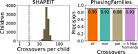
We ran our crossover detection method on GATK-called variants from the 17-member family of the platinum genome NA12878. This three-generation family has been sequenced using two sequencing technologies and six variant calling pipelines (Eberle et al. 2017) to eliminate variant calling errors and to detect crossovers. We ran PhasingFamilies on one generation of the family, composed of NA12878, her husband, and 11 children. PhasingFamilies correctly identified IBD status of siblings in a median of 99.8% of the genome and achieved a precision of 0.81 and recall of 0.97 on crossover calls, as shown in Figure 1.
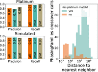
Precision and recall of PhasingFamilies on the NA1281 platinum family and simulated genomes. At top left, we identify crossovers in the 11 children of NA12878 using PhasingFamilies and compare them to crossovers detected by Eberle et al. (2017). PhasingFamilies shows high recall. Its precision is significantly higher on paternal crossovers than maternal crossovers. At right we show that many of the crossovers called by PhasingFamilies but not Eberle et al. (2017) are very close to other crossovers. Next we simulated 100 children with known crossover locations using genetic data from the NA1281 family. At lower left, we see that PhasingFamilies shows high precision and recall on this simulated data.
Precision was significantly higher for paternal crossovers than maternal crossovers (P-value = 0.003 by chi-squared test). Furthermore, 60% of the crossovers called by PhasingFamilies but not Eberle et al. (2017) were within 1 Mbp of another crossover as shown in Figure 1. These crossovers may be spurious, but they also may be the result of complex crossover or noncrossover events, which are known to occur more frequently during female meiosis (Halldorsson et al. 2016). These events are difficult to definitively detect because they contain alternating stretches of variants from each chromosomal copy and can extend >100 kbp in length (Halldorsson et al. 2019), creating potential false negatives in the platinum genome crossover callset and distorting the precision of PhasingFamilies. After excluding crossovers within 1 Mbp of another crossover, precision rose to 0.91.
Validating PhasingFamilies with simulated data
To bypass the challenge of complex crossover and noncrossover events, we simulated children from the NA1281 family with known crossover locations. Using these simulated children, PhasingFamilies achieved a precision of 0.93 and a recall of 0.92, with similar precision for both maternal and paternal crossovers (P-value = 0.82 by chi-squared test), as shown in Figure 1.
PhasingFamilies provides a median crossover resolution of 3.5 kbp
We resolved 167,279 maternal crossovers and 108,977 paternal crossovers using 1925 quad families from the SSC. Crossovers are resolved to the interval between SNVs, so crossover resolution is dependent both on the method and on the SNV distribution of the data set. PhasingFamilies was able to resolve crossovers to a median resolution of 3527.5 bp, whereas existing WGS-based methods (Venn et al. 2014; Halldorsson et al. 2019) resolve crossovers to a median of 5914 bp and 8752 bp, respectively, and microarray-based methods (Kong et al. 2014; Halldorsson et al. 2019) resolve crossovers to 36,704 and 33,428 bp, respectively, as shown in Figure 2. Crossover hotspots are believed to be <5000 bp in length, so better resolution of crossovers may allow us to better understand the architecture of these hotspots.
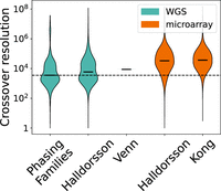
Crossover resolution. Crossovers are resolved to the interval between SNVs. Here, we compare crossover resolution for PhasingFamilies and several other methods (Kong et al. 2014; Venn et al. 2014; Halldorsson et al. 2019). Of the crossovers called by PhasingFamilies, 70.7% can be resolved to <10 kbp and 97.7% can be resolved to <100 kbp. Only the median crossover resolution was available for Venn et al. (2014).
Previous studies suggest that our two-child families should have on average 84 maternal crossovers and 56 paternal crossovers (Hussin et al. 2011). We found an average of 86.9 maternal and 56.6 paternal crossovers per family, suggesting that PhasingFamilies is able to capture nearly all genomic crossovers, with few spurious crossovers. Figure 3 shows the full distribution.
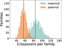
Maternal and paternal crossovers per family. Counts of maternal and paternal crossovers per family match expectations. Each family contains two children, so we expect about 84 maternal and 56 paternal crossovers per family (Hussin et al. 2011), as shown by the dotted lines.
Crossovers recapitulate existing recombination rate maps
Next, we examine the positions of our crossovers. To do this, we calculate the recombination rate in 1-Mbp intervals across the genome and compare to recent recombination rate estimates (Kong et al. 2010), produced using a HMM applied to microarray data. Recombination rates estimated from our crossovers closely match existing recombination rate maps with a Pearson correlation coefficient of 0.93 for both maternal and paternal recombination, as shown in Figure 4. Plots showing the recombination rate across the X Chromosome and all 22 autosomal chromosomes are shown in the Supplemental Figures S1 through S23.
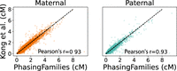
Comparison of recombination rates. We used our crossovers to produce recombination rate maps for 1-Mbp bins across the genome. PhasingFamilies produced recombination rates that correlate well with previously published (Kong et al. 2010) recombination maps.
Previous methods were unable to identify crossovers in regions within 2.5 Mbp of the chromosome ends (Kong et al. 2010), owing to limitations in the crossover-detection algorithm used. PhasingFamilies was able to identify crossovers in these regions, which is especially important on the X Chromosome, in which all paternal recombination occurs in the pseudoautosomal regions at either end of the chromosome.
Validating crossovers calls with SHAPEIT
To validate the accuracy of our crossover calls in the SSC data set, we compared them with crossovers detected using the population haplotype estimation tool SHAPEIT5 (Hofmeister et al. 2023). We ran the tool in its pedigree-aware mode and then extracted crossovers by comparing the variants inherited by each child to the phased variants in his or her parents at sites where the parent is heterozygous (for more details, see Methods). Even after filtering out crossover events that are supported by at least 100 heterozygous sites, this method produces far too many spurious crossover calls, as shown in Figure 5.
Comparison with SHAPEIT5 on Chromosome 10. The panel on the left shows the number of crossover calls per child made by the haplotype estimation tool SHAPEIT5. The dotted line indicates the number of expected crossovers on Chromosome 10, based on the median value in the platinum genome family NA1281. Although SHAPEIT5 produced far too many false-positive crossover calls to evaluate recall, we were able to validate the precision of PhasingFamilies, as shown in the right panel. Precision was significantly higher for maternal crossovers than for paternal crossovers.
Although the high rate of spurious calls made it impossible to validate recall, we were able to use the SHAPEIT5 crossovers to validate the precision of PhasingFamilies as shown in Figure 5. PhasingFamilies showed significantly higher precision on maternal crossovers than paternal crossovers (P-value 1 × 10⁻¹⁶ by chi-squared test). We believe this is owing to the high-confidence threshold we applied to the SHAPEIT5 crossovers, which inadvertently removed crossovers near the ends of the chromosome. Because male meiosis tends to produce more crossovers near chromosome ends (Sardell and Kirkpatrick 2020), this artificially deflated precision. To support this hypothesis, we calculated the precision of crossovers >5 Mbp from the chromosome ends and noticed a marked increase in precision.
Validating sibling IBD
Sibling identity-by-descent is the amount of identical genetic material two siblings share, inherited from the same parent. Siblings should on average share 50% of their DNA. In Supplemental Figure S24, we look at the fraction of maternal and paternal genetic material shared IBD by the sibling pairs in our data set. We see that the distribution of IBD matches the expected distribution. Maternal IBD is expected to have lower variance than paternal IBD primarily because maternal meiosis produces nearly twice as many crossovers as paternal meiosis. As expected, maternal and paternal IBD are not correlated as shown in Supplemental Figure S25.
Validating inherited deletions
To validate the inherited deletions detected by PhasingFamilies, we used the gold-standard structural variant calls for HG002, one member of a trio from the Genome in a Bottle (GIAB) Consortium. We also used aCGH data available for 159 families in the SSC (Levy et al. 2011).
PhasingFamilies identified 93 inherited deletions for HG002. Comparing these deletions to the gold-standard structural variant calls for HG002, we find that the precision and recall of PhasingFamilies for the HG002 trio is 0.886 and 0.074, respectively, as shown in Figure 6. The excellent precision of PhasingFamilies indicates that the majority of the inherited deletions we detect are true deletions. The precision of our deletion calls increases for longer deletions. The low recall of PhasingFamilies indicates that there are many deletions this method was not able to detect. This is expected because PhasingFamilies works only with variant calls so is unable to detect deletions that do not have any SNVs within the span of the deleted region. Recall increases both for longer deletions and for deletions with more SNVs within the deleted region. A single SNV does not make a big impact, but if the deletion spans 20 or more SNVs, recall is markedly improved to about 0.5. Larger deletions are more likely to contain many SNVs within the span of the deletion, making them easier to identify from variant patterns in the family.
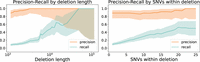
Precision and recall of inherited deletions for HG002. Inherited deletions detected by PhasingFamilies show high precision, with recall dependent on the length of the deletion. As deletion length increases, recall increases from 0.082 to 1.0, as shown in the left panel. Recall also improves with more SNVs within the deleted region, as shown in the right panel. Shaded regions indicate the Agresti–Coull binomial confidence interval.
Although gold-standard data sets like HG002 are very useful for benchmarking, they have many limitations. Out of necessity, calls are only made in well-behaved regions of the genome, excluding structural variants in so-called “dark” areas of the genome where reads cannot be assembled or aligned well. Deletions in these regions may still be highly relevant to disease (Ebbert et al. 2019) but are not evaluated when using gold-standard benchmarks. Furthermore, because of the small number of gold-standard structural variant data sets, callers may overfit to a handful of data sets, making it difficult to accurately compare performance between callers (Cameron et al. 2019).
To address this, we further verify the precision of our deletion calls using aCGH data, available for a portion of the SSC samples. We identified 71,042 deletions in the SSC data set ranging from 1 kbp to 1.3 Mbp in size. Children inherited a median of 396 kbp of deletions from their mothers and 373 kbp from their fathers. The distributions of maternal and paternal deletions were largely similar. We used aCGH to validate deletions containing more than two aCGH probes, which represent 54.6% of the deletions called by PhasingFamilies. Using aCGH to validate these deletion calls, we find that PhasingFamilies has a precision of 0.833, as shown in Supplemental Figure S26, with precision increasing with deletion length.
Discussion
We have introduced a method for detecting crossovers and shared genetic material in families, which we call PhasingFamilies. This method is not limited to WGS data. Rather, it can be applied to any type of sequencing data including whole-genome, whole-exome, or microarray data. PhasingFamilies handles the complexities presented by WGS data by identifying error-prone regions of the genome and by modeling inherited deletions. PhasingFamilies requires only two-generation pedigrees, readily scales to large data sets, can be parallelized both by family and by chromosome, and does not require manual filtering of spurious crossovers. In a large cohort of 1932 quad families, PhasingFamilies detected crossover events with a median crossover resolution of 3.5 kbp. We validated PhasingFamilies with a variety of independent data sets and techniques.
However, PhasingFamilies has several limitations. Because we use family structure to identify crossovers, we require families to have at least two children in order to identify crossovers. Runtime and memory usage are exponential in the size of the family, making families with up to seven members computationally tractable. In most family data sets, this limitation is not a major issue. In this project, our data set contained only quads.
Another limitation stems from the fact that PhasingFamilies uses variant calls produced by aligning reads to a reference genome. This means we cannot detect crossovers in regions corresponding to gaps in the reference. For reference GRCh38, which was used for most of the results in this paper, the short arms of the acrocentric chromosomes are gaps, as are the areas around the centromeres, with large centromeric gaps on Chromosomes 1 and 9. The performance of our algorithm should increase as gaps in the reference are closed, particularly as the recently released Telomere-to-Telomere Consortium genome (Nurk et al. 2022) is incorporated into the reference.
Finally, the crossover resolution of any family-based method depends on the density of SNVs around crossover breakpoints. This makes it challenging to compare the performance of different methods run on different data sets. The adoption of a gold-standard data set would make it easier to compare performance across methods. We propose using the third-generation, 17-member NA1281 family for this purpose. We make our crossover calls for this family available as Supplemental Data S4 so that others can use them for comparison.
Genetic data from families provide unique opportunities to identify and study crossover events, as well as shared genetic material in families. In fact, using genetic data from families is one of the only ways to identify individual crossover events. We provide an open-source tool to identify these events in any type of genetic data, including microarray or high-throughput sequencing data.
Methods
Detecting inheritance of shared genetic material
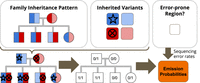
Every child in the family has two copies of each autosomal chromosome, one inherited from mom and one from dad, as shown in Figure 7. We model, much like existing methods for detecting recombination events in families (Roach et al. 2010), the observed variant calls as a Markov process with each state representing the inheritance pattern of all of the children in the family. However, we extend the state space to capture the presence or absence of inherited deletions on any of the four parental copies of the chromosome. We also extend the state space to flag error-prone regions of the genome. PhasingFamilies is able to simultaneously (1) find crossover events in children, (2) capture error-prone regions in the genome, (3) identify inherited deletions, and (4) detect which parent the deletion was inherited from.
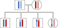
Family inheritance patterns. Each child inherits one copy of each autosomal chromosome from both parents. However, these copies are not exact replicas of either parent's chromosomes. Instead, recombination events produce a mixture of each parent's two copies. In this figure, darker and lighter blue represent the paternal copies, and red and pink represent the maternal copies.
PhasingFamilies assumes that the input data are not phased. The input to our algorithm is a VCF file containing genetic data along with a PED file specifying familial relationships. We do not incorporate population allele frequency. We rely solely on variant transmission patterns within the family. PhasingFamilies produces crossover calls and inheritance patterns for any families containing two or more children.
Although PhasingFamilies can be applied to trios in order to phase variants in the child or to detect inherited deletions, PhasingFamilies (and any family-based method) cannot detect crossovers in a trio, as shown in Supplemental Figure S27.
Next we define our model by describing the state space, transition probabilities, and emission probabilities.
State space
Each state in our model captures three types of information as shown in Figure 8. First, the family inheritance pattern defines which parental copy is inherited by each child in this state. Second, the inherited variants represent the variants on each parental copy, with options of SNV variant, no variant, or deletion variant. Third, the error-prone region flag indicates whether this state represents an error-prone region of the genome, for example, a centromeric region or a region with repetitive sequence.
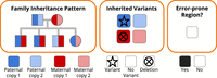
Hidden Markov model (HMM) state space. The state space of our HMM defines the family inheritance pattern, the presence of deletions and SNVs, and whether or not the genomic region is error-prone.
Transition probabilities
Next, we define the transition probabilities of our model. Transitions can represent crossover events or the beginning or end of a deletion or an error-prone region. We assume all of these events are independent, so when calculating the transition probability between two states, we look at all of the ways the states differ and multiply the probabilities of these various events together.
A transition between states with different family inheritance patterns represents a recombination event in one or more of the children. Recombination events are known to be rare, with an estimated 22.8 paternal crossover events genome-wide per child (Wang et al. 2012) and 1.7× more maternal crossover events than paternal (Petkov et al. 2007). To reflect this, we set the probability of a paternal crossover to be 22.8/G and the probability of a maternal crossover to be 22.8 × 1.7/G, where G is the length of the human genome.
A transition between states with different inherited variants represents either an entry or exit from an inherited deletion or a change in the presence or absence of SNV variants. We estimate approximately 102 detectable inherited deletions per parental genome copy, each with an entry and exit defined by a state transition, so we assign the probability of transitioning into or out of a deletion to be 2 × 10²/G. To make this estimation, we counted the number of inherited deletions in the HG002 trio containing at least five SNVs, which is on the order of 102. We experimented with different values and found that our model is quite robust to the choice of this parameter. We assume that SNV variants occur randomly and that the presence of an SNV at one position is independent of the presence of an SNV at another, so we assign equal transition probabilities between states with any configuration of inherited SNV variants.
The error-prone region flag is used to identify areas of the genome where the family contains many variant calling errors. A transition between states with different error-prone region flags indicates a transition into or out of one of these error-prone regions of the genome. We estimate approximately 103 error-prone regions per parental genome, so we assign the probability of transitioning into or out of an error-prone region to be 2 × 10³/G. To make this estimation, we counted the number of low-complexity regions (Li and Wren 2014) containing at least five SNVs, which is on the order of 103. We experimented with different values and found that our model is quite robust to the choice of this parameter.
Emission probabilities
Each state completely defines the expected genotypes of every family member, as shown in Figure 9. We expect variants to be inherited by the children according to the family inheritance pattern. Deletion variants are also
inherited according to the family inheritance pattern, producing distinctive variant call patterns owing to hemizygous variants,
as shown in Supplemental Figure S28. The existence of error-prone regions of the genome is captured by the error-prone region flag. States with this flag show
higher error rates for all individuals. We assume variant calling errors are independent across family members, so if there
are m family members, then the emission probabilities for state s with expected genotypes (g1, g2, …, gm) and error-prone region flag e are  for every combination of family variant calls (v1, v2, …vm).
HMM emission probabilities. Emission probabilities represent the probability of observing a set of family variant calls given that we are in a particular state. To estimate these probabilities, we first use the family inheritance pattern and the inherited variants to calculate the expected genotypes for the family. We then use the error-prone region flag to determine which set of variant calling error rates to use for the state. Finally, we calculate the emission probabilities for the state.
We estimate the rate of variant calling errors for each individual in the family using a published method based on Poisson regression (Paskov et al. 2021). This method estimates variant calling error rates for each individual in a family using Mendelian errors. The method can be applied either genome-wide or to specific genomic regions in order to estimate error rates within these regions.
For our model, we require two sets of variant calling error probabilities: one for error-prone regions and another for the rest of the genome. To calculate the variant calling error rate for error-prone regions, we use the low-complexity regions described by Li and Wren (2014) and generated by the mdust program. We restrict our Poisson regression to only consider variants in these regions, in order to accurately estimate variant calling error rate for each sample within error-prone regions of the genome. Supplemental Figure S29 shows the emission probabilities calculated for our cohort.
Using problem structure to efficiently implement the Viterbi algorithm
Given a fully defined HMM, the Viterbi algorithm (Forney 1973) finds the path through the state space that best explains the observed variant calls, as shown in Supplemental Figure S30.
We start by computing the computational cost of a naive Viterbi implementation. If we have m members in our family, then our state space has size p = 22(m−3) × 34 × 2. The first term represents the number of possible inheritance patterns. Mom has maternal copy 1 (m1) and maternal copy 2 (m2); dad has paternal copy 1 (p1) and paternal copy 2 (p2); and we fix the first child to inherit m1 and p1 in order to prevent symmetrical solutions for small families. The second term represents the number of possible inherited variant combinations for each of the four parental chromosomes. Finally, the third term represents the error-prone region flag.
If a chromosome is n positions long, and we have p state spaces, then the Viterbi algorithm will require O(np2) operations. Because we are working with a state space that is exponential in the number of family members, the p2 term in our runtime is problematic. To address this, we restrict the transitions we allow between states so that we allow only a single crossover event per position. This is biologically plausible because we expect very few crossover events per child (on the order of one per chromosome), and it is extremely unlikely that two children would have crossovers at the same position (Wang et al. 2012). This means that during the forward pass of the Viterbi algorithm, we need only consider 2(m − 3) × 34 × 2 previous transitions for each state, making our runtime O(pmn). This runtime is still exponential in the number of individuals in the family, but this exponential factor is no longer squared.
We can also decrease n by observing that at most positions in the genome, all family members will have homozygous reference. These positions are uninformative with respect to the inheritance pattern of the family as well as the presence or absence of inherited deletions. We can therefore limit our algorithm to consider only positions where at least one family member has a variant. This decreases n by a factor of around 1000×. Our model is focused on capturing crossovers, which are both rare and typically far apart (Otto and Payseur 2019), so we can assume that many variants will occur between any two crossovers and, therefore, that removing positions where all family members are in homozygous reference will not require a change in the transition matrix.
Compute time
Our algorithm scales linearly with chromosome length, as shown in Figure 10. It scales exponentially with family size but has very reasonable runtimes for families with five or fewer children. The median runtime for WGS data from a family of four on Chromosome 1 is 4.6 min.
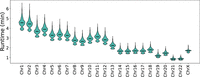
Algorithm runtime. Our algorithm scales linearly with chromosome size. The median runtime for WGS data from a family of four on Chromosome 1 is 4.6 min, making it efficient enough to be applied to large cohorts.
Uncertainty regions
The Viterbi algorithm identifies the maximum likelihood path through state space, given the observed data. However, if two paths have nearly identical likelihood, for example, a crossover event occurs somewhere in a stretch of homozygosity, as shown in Figure 11, then rather than arbitrarily choosing one of the two paths, we mark the region as uncertain. We do this during the backward Viterbi sweep by marking any regions where multiple paths are within 1/10 of the maximum likelihood path as uncertain. We selected this threshold empirically.
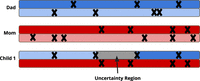
Uncertainty regions. Because of long stretches of homozygosity in families, it may be difficult to determine exactly where a crossover event occurs.
Determining crossover resolution
Because of the uncertainty regions described above, we can only rarely determine the exact base pair where a crossover event occurs. Instead, we can use our model to determine that a crossover event occurred somewhere within a stretch of homozygosity bordered by two SNVs. When we discuss the resolution of a crossover, we mean the distance between these two SNVs.
De novo variants
We chose not to directly model de novo variants because they are so rare compared with the sequencing error rate for WGS data. De novo variants would be interpreted by our algorithm as sequencing errors.
Algorithm output
Our code produces the following outputs (file format in parentheses): inheritance patterns (BED), crossovers (JSON), noncrossovers (JSON), genome wide IDB for sibling pairs (JSON), chromosomal IBD for sibling pairs (JSON), inherited deletions (JSON), and error-prone regions (JSON).
Our algorithm does not directly produce per-family phased haplotype blocks, although they could easily be reconstructed from the inheritance pattern files and variant calls. The haplotype blocks identified by our algorithm are quite large because they are defined by crossovers within the family, with a median haplotype block size of 23,349,429 bp for maternal crossovers and a median haplotype block size of 38,155,890 bp for paternal crossovers in SSC, as shown in Supplemental Figure S31.
WGS data sets
We applied PhasingFamilies to WGS data from 1932 quad families, each with two children (one affected child and one unaffected sibling) from the SSC (Turner et al. 2017). Data are available at https://www.sfari.org/2017/08/22/whole-genome-sequencing-of-the-simons-simplex-collection-new-data-release/.
Each individual was sequenced at 30× coverage using an Illumina PCR-free library protocol. Reads were aligned to build GRCh38 of the reference genome using BWA-MEM (Li 2013) v0.7.8, and variants were called using GATK (Poplin et al. 2018) v3.5. Only biallelic variants that pass the VQSR step of the GATK were included in analysis. The joint VCF file was then passed into PhasingFamilies. We used these families to validate crossovers and IBD among families.
We also applied PhasingFamilies to the NA12878 platinum genome, along with her spouse and 11 children to validate crossover calls. Crossover locations for the 11 children have been called using two sequencing technologies and six variant calling pipelines (Eberle et al. 2017). We pulled all biallelic SNPs called using the bwa-gatk pipeline from three VCF files: High_Confidence_Calls_HG19.vcf.gz, manuscript_supplement_filtered_ped_consistent.vcf.gz, and manuscript_supplement_hq_fails.vcf.gz. By merging variants from all three files, we generate a family VCF that includes variant calling errors, so that we can evaluate the performance of our crossover detection method in the presence of variant calling errors.
We also applied PhasingFamilies to the HG002 trio (Zook et al. 2016). Each individual was sequenced at 60× coverage with a median fragment length of 555 bp. We used the standard GATK pipeline to call variants. The joint VCF file produced by GATK was then passed into PhasingFamilies. HG002 is a GIAB Consortium sample with gold-standard structural variant calls that are widely used to estimate the performance of structural variant callers (Cameron et al. 2019). We used this family to validate the inherited deletions detected by our model.
Identifying identical twins, unrelated individuals, and other outliers
After determining inheritance patterns in families using our HMM, it is important to identify sibling pairs with unusual relationships. For example, siblings may be identical twins, or owing to errors in the PED file, two individuals labeled as siblings may in reality be half-siblings or unrelated individuals. To identify these unusual relationships, we use Gaussian kernel density estimation to detect IBD outliers. We first calculate maternal and paternal IBD between all sibling pairs in our data set, and then we run our outlier detection algorithm to label siblings that either share too much genetic material (identical twins) or too little (PED file errors). In our SSC cohort, three families (out of 1932) were filtered out owing to being IBD outliers.
Removing spurious crossover events
The high error rate of WGS data can easily lead to spurious crossover calls. We avoid this using the error-prone regions detected by our HMM. If a crossover occurs within an error-prone region, we use the boundaries of the error-prone region as the uncertainty boundaries of the crossover. This eliminates a huge number of spurious crossover calls, as shown in Supplemental Figure S32. It also produces a small number of crossovers with very large resolutions (>1 Mbp), owing to large error-prone regions, as shown in Supplemental Figure S33.
We also use Gaussian kernel density estimation to detect crossover outliers. We first calculate the number of maternal and paternal crossover events for each sibling pair in our data set, and then we run our outlier detection algorithm to label siblings with too many or too few crossovers. In our SSC cohort, four families (out of 1932) were filtered out owing to being crossover outliers.
Filtering potential noncrossover events
Noncrossover events (also known as gene conversions) occur when a double-stranded break is resolved not with a crossover, but with a small section of genetic material being copied from one homologous chromosome to the other. These noncrossover events are short; however, PhasingFamilies should be able to detect them provided a sufficient number of SNVs fall within the copied region.
We detect and filter out potential noncrossover events when two inheritance pattern transitions occur for the same child within 161,332 bp of each other if the transitions are both maternal or within 154,265 bp of each other if the transitions are paternal. These cutoffs are derived from the Simons SPARK data set Feliciano et al. (2018), containing 3239 families and 13,248 individuals. We applied our algorithm, calculated the distance between all inheritance pattern transitions for each child, and took the 1% quantile for maternal and paternal transitions, respectively. Potential noncrossover events are output to a JSON file.
Validating PhasingFamilies with the NA1281 platinum genome family
We used the NA12878 platinum genome, along with her spouse and 11 children to validate PhasingFamilies. Crossover locations for the 11 children have been called using two sequencing technologies and six variant calling pipelines (Eberle et al. 2017). We broke the family into quads in order to evaluate the performance of PhasingFamilies when only two children are available. We then ran our crossover detection algorithm on these quad families.
We then compared the crossovers detected by PhasingFamilies to those detected by Eberle et al. (2017). We considered a crossover validated if the crossover was within 105 bp of a crossover in the validation callset.
Simulating genomes with known crossover locations
To validate PhasingFamilies, we simulated genomes using the NA12878 platinum genome and her family. We simulated children of NA12878 and her spouse by randomly selecting two real children: one to use as a maternal haplotype model and the other to use as a paternal haplotype model. We then pulled the maternal inheritance pattern for the first child and the paternal inheritance pattern for the second, and we randomly inverted each with a probability of 0.5. This gave us a new inheritance pattern for our simulated child with known maternal and paternal crossover locations (drawn from the maternal and paternal haplotype model children, respectively). At each position on Chromosome 10, we generated variant calls for our new simulated child by randomly selecting the variant call of a real child who shared the same inheritance pattern at that position with the simulated child. We generated 100 simulated children in this way and then ran our crossover detection algorithm on this simulated data.
We then compared the crossovers detected by PhasingFamilies to the known locations of maternal and paternal crossovers in the simulated genomes. We considered a crossover validated if the crossover is within 105 bp of a crossover in the validation callset.
Validating crossover calls with SHAPEIT
We used SHAPEIT5 (Hofmeister et al. 2023) to validate the precision of our crossover calls. The primary goal of SHAPEIT5 is haplotype estimation, not crossover detection. However, crossovers can be extracted from their output by comparing the phased variants inherited by a child to the phased variants of his or her parents.
We ran SHAPEIT5 in its pedigree-aware mode on Chromosome 10 for our cohort, filtering out all variants with MAF <0.05. This produced phased variant calls for all individuals in our cohort. To extract crossovers, we compared the phased variants of a parent with their child. We called a crossover whenever the child switched from inheriting the parent's paternal variant (listed first in the phased genotype) to inheriting the parent's maternal variant (listed second in the phased genotype) or vice versa. We then filtered these crossover calls based upon how many informative positions supported the inheritance pattern on either side of the crossover. Supplemental Figure S34 shows the number of crossovers called depending upon the number of informative positions required. In all cases, this method produced far too many crossover calls. Even after requiring at least 100 informative positions on each side of the crossover, many spurious crossovers remain (median is 48 crossovers per child, when only about three are expected for Chromosome 10). This high rate of spurious crossovers made it impossible to validate the recall of PhasingFamilies; however, we were able to validate precision. We considered a crossover validated if the crossover is within 105 bp of a crossover in the validation callset.
Validating inherited deletions
To estimate the precision and recall of the inherited deletions detected by PhasingFamilies, we ran the method on the HG002 trio and compared the inherited deletions identified using PhasingFamilies to the gold-standard deletion set provided for sample HG002 (Zook et al. 2020).
When comparing our deletions to the gold standard, we first discard any deletions whose endpoints fall outside of the known high-confidence regions (Zook et al. 2016). Because PhasingFamilies focuses on identifying inherited deletions, we also discard any HG002 gold-standard deletion calls with the Mendelian error flag. Finally, we restricted our analysis to deletions >1 kbp long. There are 801 deletions in the HG002 gold-standard SV calls that meet these requirements. We consider a deletion validated against the HG002 gold-standard calls if the deletion overlaps an HG002 gold-standard deletion and the overlap is at least 50% of the length of both deletions, a standard metric.
To further examine the precision of our deletion calls, we use aCGH data available for 628 individuals in the SSC (Levy et al. 2011). The aCGH assay is a microarray-based method for analyzing ploidy-level differences between the DNA of a sample and a reference, producing a continuous output. Although methods exist for detecting deletions or duplications based on aCGH output (Levy et al. 2011), here we focus on validating the deletions detected by PhasingFamilies by evaluating the aCGH output of probes within the span of the deletion. In particular, we work with the LOWESS of local ratio of aCGH probe intensities, a commonly used normalization framework for aCGH data (Khojasteh et al. 2005). We evaluate all deletions called by PhasingFamilies that contain more than two aCGH probes. We consider a deletion validated if either (1) the median LOWESS of local ratio, computed against the reference sample, across all probes within the span of the deleted region, is <0.84; or (2) the median LOWESS of local ratio, computed with respect to the parent who did not transmit the deletion, across all probes within the span of the deleted region, is less than 0.84.
The cutoff of 0.84 was determined by plotting the median normalized aCGH value for every deletion with at least two aCGH probes and by choosing the lowest point between the two peaks corresponding to reference-level and deletion-level ploidy, as shown in Supplemental Figure S35.
This procedure allows us to use aCGH data to validate the precision of PhasingFamilies, but it does not allow us to validate recall. To validate recall using aCGH, we would need to run a deletion-detection algorithm on the aCGH data in order to identify deletions that were not detected by PhasingFamilies. This method itself might produce spurious deletions or might miss real deletions, both of which would make our estimated recall inaccurate. In particular, aCGH data are microarray based, so cannot detect very small deletions. For this reason, we chose to validate recall with the HG002 sample. The gold-standard deletion callset available for HG002 was produced from a variety of sequencing techniques including short-read, linked-read, and long-read sequencing, as well as optical mapping (Zook et al. 2020), making it more suited to measuring recall.
Data access
All crossovers detected in the SSC data set are available as Supplemental Data S1. The 1-Mbp maternal and paternal recombination rate maps generated from SSC are available as Supplemental Data S2 and Supplemental Data S3. Crossovers detected in the platinum genome family NA12871 are available as Supplemental Data S4. The code generated for this study is available at GitHub (https://github.com/kpaskov/PhasingFamilies) and as Supplemental Code.
Competing interest statement
The authors declare no competing interests.
Acknowledgments
We acknowledge funding from the Hartwell Foundation, the Bio-X Center, and the Precision Health and Integrated Diagnostics Center. We acknowledge the Simons Foundation for collecting and making available genetic data from the Simons Simplex cohort. We thank all of the families at the participating Simons Simplex Collection (SSC) sites, as well as the principal investigators (A. Beaudet, R. Bernier, J. Constantino, E. Cook, E. Fombonne, D. Geschwind, R. Goin-Kochel, E. Hanson, D. Grice, A. Klin, D. Ledbetter, C. Lord, C. Martin, D. Martin, R. Maxim, J. Miles, O. Ousley, K. Pelphrey, B. Peterson, J. Piggot, C. Saulnier, M. State, W. Stone, J. Sutcliffe, C. Walsh, Z. Warren, and E. Wijsman). We appreciate obtaining access to genetic data on SFARI Base.
Footnotes
-
[Supplemental material is available for this article.]
-
Article published online before print. Article, supplemental material, and publication date are at https://www.genome.org/cgi/doi/10.1101/gr.277172.122.
- Received August 2, 2022.
- Accepted September 12, 2023.
This article is distributed exclusively by Cold Spring Harbor Laboratory Press for the first six months after the full-issue publication date (see https://genome.cshlp.org/site/misc/terms.xhtml). After six months, it is available under a Creative Commons License (Attribution-NonCommercial 4.0 International), as described at http://creativecommons.org/licenses/by-nc/4.0/.


