
Abstract
Spatial omics (SOs) are powerful methodologies that enable the study of genes, proteins, and other molecular features within the spatial context of tissue architecture. With the growing availability of SO data sets, researchers are eager to extract biological insights from larger data sets for a more comprehensive understanding. However, existing approaches focus on batch effect correction, often neglecting complex biological patterns in tissue slices, complicating feature integration and posing challenges when combining transcriptomics with other omics layers. Here, we introduce spatial multislice/omics analysis (stMSA), a deep graph contrastive learning model that incorporates graph auto-encoder techniques. stMSA is specifically designed to produce batch-corrected representations while retaining the distinct spatial patterns within each slice, considering both intra- and inter-batch relationships during integration. Extensive evaluations show that stMSA outperforms state-of-the-art methods in distinguishing tissue structures across diverse slices, even when faced with varying experimental protocols and sequencing technologies. Furthermore, stMSA effectively deciphers complex developmental trajectories by integrating spatial proteomics and transcriptomics data and excels in cross-slice matching and alignment for 3D tissue reconstruction.
Spatial omics (SO) technologies have greatly enhanced our understanding of molecular expression and interactions within tissue architectures (Williams et al. 2022). These methodologies allow for the simultaneous analysis of thousands of genes, proteins, or metabolites, revealing their precise spatial distribution in tissues. Spatial transcriptomics (STs) are a leading technique in this field, providing detailed views of the transcriptome in spatial perspective (Asp et al. 2020). Recently, cellular indexing of transcriptomes and epitopes by sequencing (spatial CITE-seq) (Liu et al. 2023) has emerged as a significant advancement in SOs. This technique integrates RNA sequencing with the measurement of surface protein expression using specific antibodies, thereby enriching transcriptomic data with valuable spatially resolved proteomic information. This integration allows for a comprehensive understanding of the spatial distribution of proteins, offering invaluable insights into the proteomic landscape within tissues. These advancements have paved the way for novel applications in understanding cellular interactions, identifying spatial biomarkers, and unraveling complex developmental and disease processes (Cheng et al. 2023).
In tandem with the evolution of SO technologies, numerous computational methods have been proposed to analyze individual slices. A critical step in these analyses is the identification of spatial domains, which involves clustering spots with similar molecular expression profiles and spatial locations in an unsupervised manner. Accurate integration of molecular expression and spatial information is essential for this process. For instance, STAGATE (Dong and Zhang 2022) utilizes self-attention mechanisms and cell type–aware spatial graphs to learn latent representations of spots, whereas CCST (Li et al. 2022) employs a Deep Graph Infomax (DGI) model, providing a general framework for multiple ST analysis tasks, including spatial domain detection and cell cycle identification. Although these methods have successfully analyzed individual slices, they remain limited to two-dimensional (2D) analyses owing to their single-slice focus.
As the availability of SO data derived from the same tissues, organs, or embryos increases, there is a growing need to integrate multiple slices (Schott et al. 2024). When slices are oriented horizontally, this integration facilitates extended spatial analyses; when vertical, it enables the reconstruction of three-dimensional (3D) models that more accurately reflect true spatial structures and cellular functions. Although some methods, such as Scanorama (Hie et al. 2019) and Harmony (Korsunsky et al. 2019), have been adapted for integrating SO data, their performance is often limited owing to inadequate utilization of spatial information (Yue et al. 2023). Methods like SEDR (Xu et al. 2024) address batch effects by learning latent representations for each slice using deep autoencoders; however, they overlook cross-slice relationships. Recently proposed methods, such as STAligner (Zhou et al. 2023) and STitch3D (Wang et al. 2023), specifically aim to integrate multiple SO slices but still encounter limitations. For instance, STAligner employs mutual nearest neighbors (MNNs) for integration, whereas STitch3D requires additional reference data that can impact performance. Moreover, there are currently no effective methods for integrating spatial multiomics data, such as combining transcriptomics with proteomics, to reveal intricate biological patterns from both perspectives.
To address these challenges, we present stMSA, a novel graph contrastive learning–based method with a core aim: integrating SO data from multiple sources. stMSA employs a contrastive learning strategy, optimizing two key principles to simultaneously learn the embeddings of cross-batch spots. First, within each slice, the embeddings of spots in connected adjacent spatial niches are made similar, whereas those of randomly sampled spots remain dissimilar. Second, embeddings of cross-batch spots with similar gene expression profiles are optimized to be similar, whereas those of randomly sampled cross-batch spots diverge. By adhering to these principles, stMSA enables joint spatial domain identification across slices, cross-slice spatial matching for correspondence inference, and multislice alignment for 3D tissue reconstruction. By unifying these capabilities, stMSA facilitates integrative analysis of spatially resolved multiomics data, advancing insights into complex tissue architectures.
Results
Overview of stMSA
This study introduces stMSA, a novel deep graph representation learning model designed for integrating multiple SO data (Fig. 1A). The primary objective of stMSA is to generate consistent cross-batch spot embeddings, essential for tasks such as joint domain detection, cross-slice matching, and 3D reconstruction alignment (Fig. 1B).
Overview of the stMSA framework. (A) stMSA leverages multislice omics expression and spatial coordination information as input. It utilizes an auto-encoder to learn latent batch-corrected multislice representation and optimizes the model through three distinct optimization tasks. (B) The latent embedding learned by stMSA serves various downstream tasks, including multislice domain detection, cross-slice tissue structure identification, multiplatform integration, cross-slice matching, and multislice alignment.
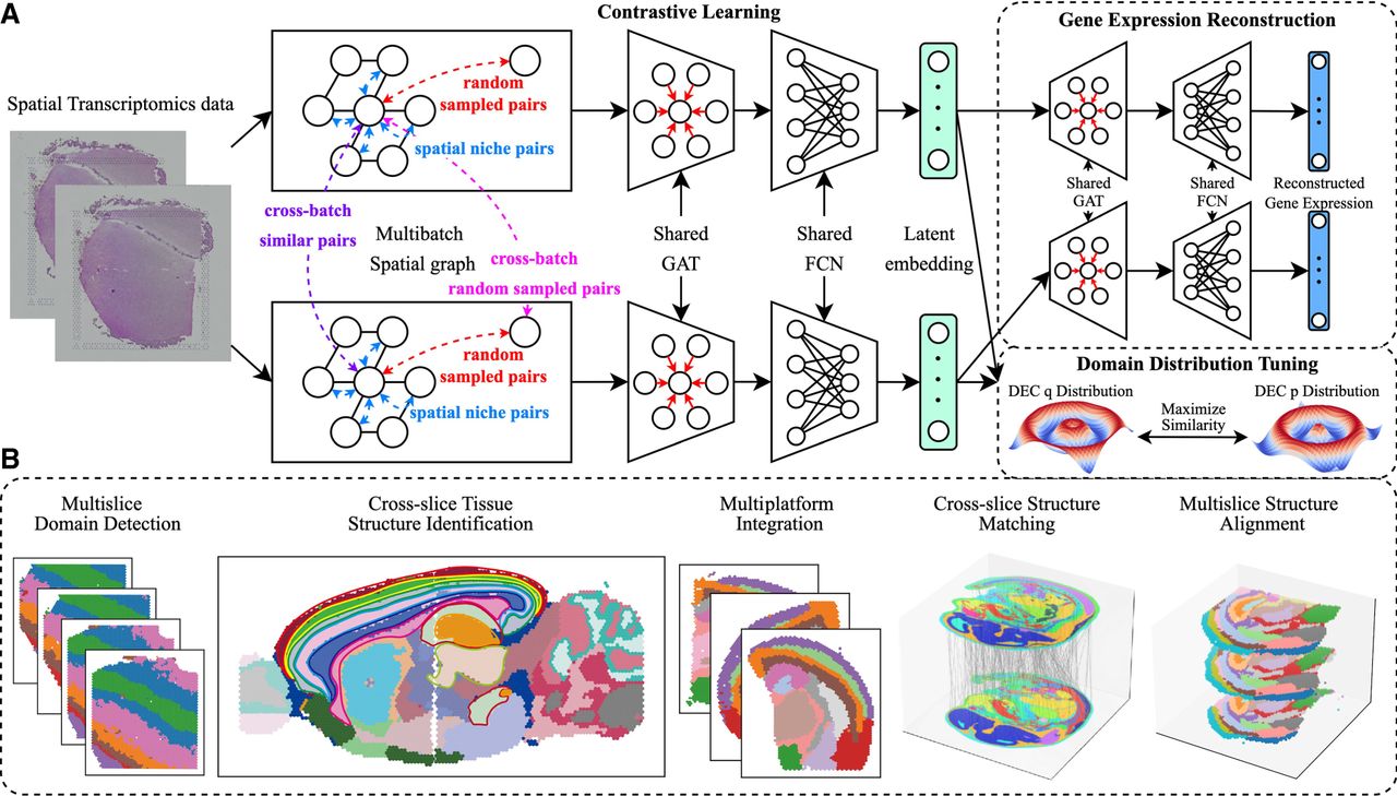
The model processes preprocessed omics expression data and spatial information from multiple slices as input. For each slice, stMSA constructs a spatial graph using the coordinates of each spot. It then utilizes both the omics expression profiles and the spatial graphs to derive latent representations. The core of stMSA is a contrastive learning strategy that simultaneously considers the inner-batch patterns and the cross-batch patterns to integrate data across multiple slices. This method aims to maximize the similarity of spatially adjacent spots within the same slice and across different slices that exhibit similar gene expression patterns, while minimizing the similarity between dissimilar spot pairs, both within and between slices.
In detail, stMSA enhances the similarity between centroid spots and their associated spatial niche embedding in the latent space, enabling the model to capture detailed local features from neighboring spots. To preserve and highlight the unique expression patterns of each spot, the model also optimizes gene expression reconstruction through an attention-based graph auto-encoder, a process we term the gene expression reconstruction (GER) task. Furthermore, we refine the model's performance by dynamically optimizing the predicted spatial domains using the deep embedding clustering (DEC) method (Xie et al. 2016).
stMSA enhances joint domain identification for human dorsolateral prefrontal cortex slices
We applied stMSA to the human dorsolateral prefrontal cortex (DLPFC) data set from the 10x Visium platform (Maynard et al. 2021), which includes 12 slices from three donors with detailed spatial annotations (Fig. 2A). To assess its performance in domain identification, we compared stMSA against eight state-of-the-art methods: Scanorama (Hie et al. 2019), Harmony (Korsunsky et al. 2019), SEDR (Xu et al. 2024), STAligner (Zhou et al. 2023), Stitch3D (G Wang et al. 2023), SPACEL (Xu et al. 2023), CAST (Tang et al. 2024), and STAMP (for details, see Supplemental Note S1; Zhong et al. 2024). Domain detection performance (for visualization of full domain identification results, see Supplemental Fig. S1) was evaluated using the adjusted Rand index (ARI), normalized mutual information (NMI), completeness score (COM), and homogeneity score (HOM) for each method (Fig. 2B; Supplemental Fig. S2A).
stMSA improves joint domain identification for human dorsolateral prefrontal cortex (DLPFC) slices. (A) Manual annotations, ranging from the cortex layer 1 to the white matter, are provided with the histology image of a donor (slice identifiers: 151,507–151,510). (B) The box plot illustrates the ARI scores across 12 10x Visium DLPFC slices, generated by training separately for each donor. (C) The bar plot illustrates the average ARI scores for the two Stereo-seq DLPFC slices. Error bars represent the 95% confidence intervals of the ARI scores. Notably, STitch3D and CAST were unable to produce results for the Stereo-seq DLPFC data set on our server with 24 GB GPU memory and 128 GB RAM. (D) Visualization of domain detection results for SEDR, STAligner, Stitch3D, and stMSA. The domain detection processes are conducted using all four slices as inputs. (E) The ground-truth, STAligner, and stMSA domain detection results of the two Stereo-seq-obtained DLPFC slices. (F) The trajectory inference plot generated based on the embeddings learned by stMSA using all 12 DLPFC slices for the 10x Visium and the two Stereo-seq DLPFC slices (the color reflects the ground-truth domains). And the UMAP visualization for different donors/slices (the color reflects three donors/slices).
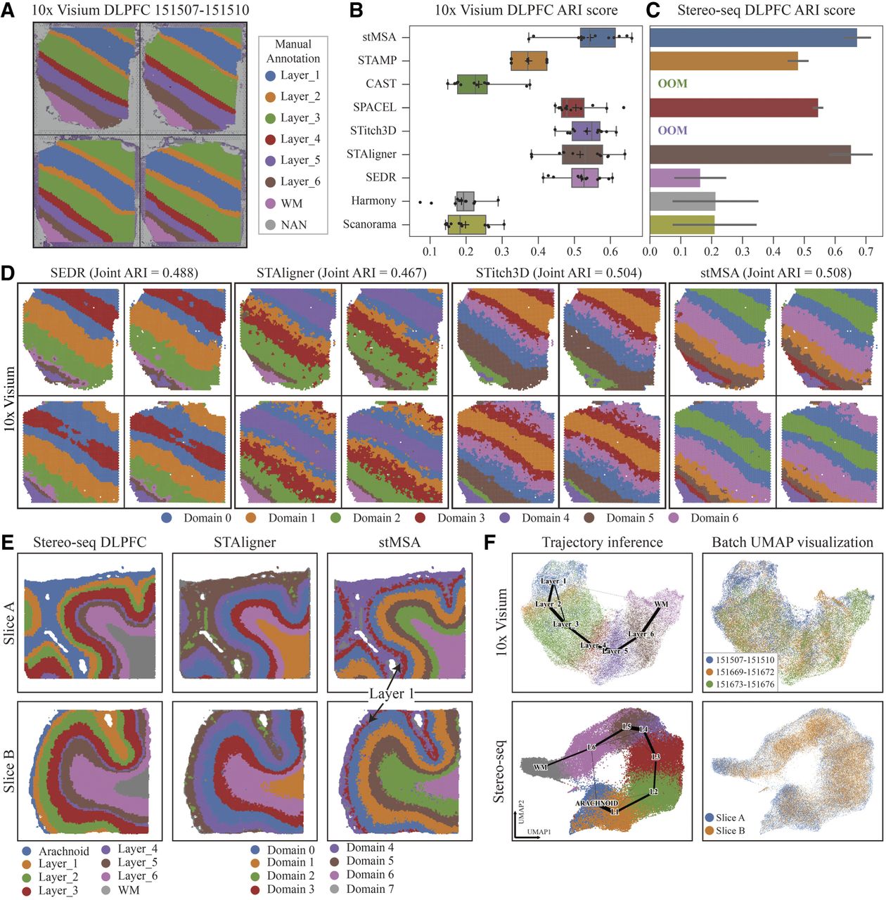
As shown in Figure 2B, stMSA achieved an average ARI score of 0.544 across 12 DLPFC slices, surpassing both STitch3D (0.535) and SPACEL (0.508). Visual comparison of spatial domain distributions for one donor (slices 151,507–151,610) further demonstrated stMSA's superior performance, achieving a joint ARI score of 0.508 (Fig. 2D). Although other top methods, such as SEDR (0.488) and Stitch3D (0.504), achieve a good ARI score, these methods showed inaccuracies in layers 2–6; stMSA produced more coherent boundaries and shapes. STAligner (0.467) was the closest competitor in spatial domain distribution but was still outperformed by stMSA in accuracy and boundary clarity.
Moreover, we assessed the sensitivity to single-cell reference data quality by cross-applying reference data sets between STitch3D and SPACEL on the DLPFC donor3 slices (151,673–151,676). Both methods exhibited reduced performance (Supplemental Fig. S2B) when using swapped references, highlighting their dependency on curated SC data for optimal accuracy.
To assess the scalability of stMSA, we applied it to two DLPFC slices from the Stereo-seq platform (Wei et al. 2025), each containing more than 30,000 spots. Comparative analysis of domain identification metrics revealed that stMSA outperformed existing state-of-the-art methods on this benchmark data set evaluated by the domain prediction accuracy metrics (Fig. 2C; Supplemental Fig. S2). Moreover, stMSA, STAligner, SPACEL, and STAMP represented the layer structures well, whereas other methods failed to capture the zonal domains (Fig. 2E; Supplemental Fig. S3). Trajectory analyses (Wolf et al. 2019) confirmed that stMSA effectively traced the path from white matter to the arachnoid membrane (Fig. 2F), unlike Scanorama, Harmony, and SEDR, which conflated multiple layers. Notably, stMSA distinguished the thin layer 1 (domain 3) from the adjacent layers, achieving the highest joint ARI score of 0.665 across two slices.
We assessed stMSA's effectiveness in removing slice-wise batch effects using UMAP visualizations (Supplemental Figs. S3, S4). The embeddings from three donors were well mixed, with no clear batch effects observed in the 10x Visium data set. This trend continued in the Stereo-seq data set, confirming successful integration across donors. Additionally, we evaluated computational efficiency. stMSA processed up to 20 slices with <12 GB of GPU memory, whereas Stitch3D, SPACEL, and SEDR struggled to handle larger data sets (Supplemental Fig. S5).
Identification of cross-batch structures using stMSA in multislice mouse brain
We applied stMSA to a sagittal section data set of the mouse brain obtained via 10x Visium sequencing, which includes multiple slices owing to the large tissue volume (Fig. 3A). Each slice, covering up to 4992 spots, was divided into anterior (Fig. 3B, left) and posterior (Fig. 3B, right) sections for analysis. Our objective was to identify common spatial domains across slices and assign consistent domain labels.
stMSA can identify cross-batch tissue structures in the 10x Visium–obtained mouse brain data set. (A) The anatomical structure of the sagittal mouse brain provided by the Allen Brain Atlas. (B) Spatial domains predicted by stMSA with manually annotated landmark domains (isocortex from layer 1 to layer 6b, hippocampus, and thalamus). (C) Subdomains of the isocortex, hippocampus, and thalamus, along with the expression levels of their corresponding marker genes. (D) The UMAP visualization of latent embeddings derived by stMSA. The substructures of the isocortex from layer 1 to layer 6b are manually annotated on the plot. (E) The anatomical structure of the coronal mouse brain provided by the Allen Brain Atlas. (F) The clustering result of stMSA in fresh-frozen with H&E-stained, DAPI-stained, and FFPE-preserved coronal mouse brain slices. (G) The ARI clustering score for stMSA and other state-of-the-art methods in the three coronal mouse brain slices.
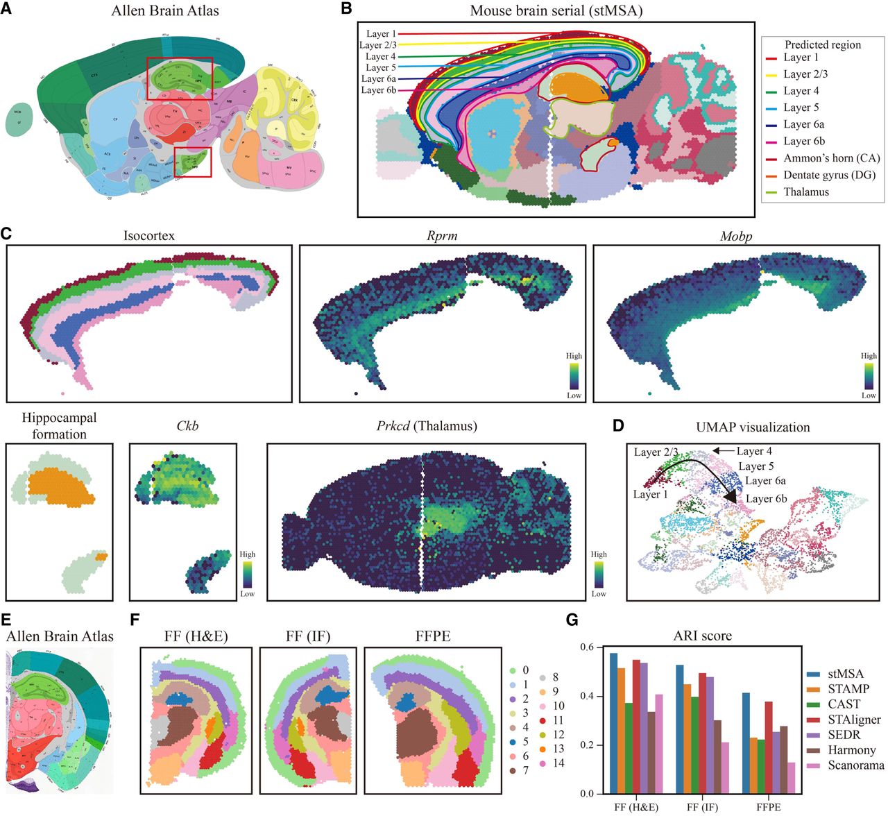
Figure 3B illustrates the domain detection performance of stMSA relative to the manually annotated structures from the Allen Brain Atlas (Fig. 3A). Moreover, we find that stMSA and STAMP can depict the cross-sections of the hippocampus and its inner subdomains well, accurately delineating the ”hook”-shaped outline of Ammon's horn. Notably, stMSA is the only method that can accurately represent cross-slice structures, including the six cortical layers in the isocortex and thalamus, whereas SEDR identified only five layers within the isocortex (Supplemental Fig. S6).
Upon further analysis of fine-grained structures, stMSA demonstrated the ability to accurately recognize subdomains within significant brain structures, such as those in the isocortex and hippocampus. Comparison of gene expression distributions with known markers confirmed the accuracy of these subdomain identifications (Fig. 3C). For example, genes like Rprm and Mobp exhibited consistent expression patterns corresponding to cortical layers (Fulcher et al. 2019; Grimstvedt et al. 2023; Hoerder-Suabedissen et al. 2023; Sullivan et al. 2023), whereas Ckb showed a ”curved tube” structure aligning with our hippocampal domain results (Sandebring-Matton et al. 2021). The spatial distribution of the marker gene Prkcd for the thalamus also significantly overlapped with structures identified by stMSA. Additionally, UMAP visualizations and trajectory inference from embeddings learned by stMSA confirmed the correspondence between the relative positions of isocortex layers and their actual physical locations (Fig. 3D; Supplemental Fig. S7).
Next, we assessed stMSA's capability to integrate coronal mouse brain data from various experimental protocols (Supplemental Note S2), including fresh-frozen tissue with H&E staining, denoted as FF (H&E); fresh-frozen tissue with immunofluorescence (DAPI) staining, denoted as FF (IF); and formalin-fixed paraffin-embedded (FFPE) tissue with H&E staining, denoted as FFPE (Supplemental Fig. S8A). stMSA standardizes inputs to preprocessed SO expression profiles across all data sets. Although auxiliary information (such as H&E/DAPI images) is available in some cases, they are intentionally excluded to ensure model generalizability and focus on core ST features. We benchmarked stMSA against state-of-the-art methods by analyzing these slices and generating embeddings in a shared feature space. Spatial domain prediction results are separately visualized for each slice to highlight method-specific performance (Fig. 3F; Supplemental Fig. S8B). Results indicated that both stMSA, STAligner, and CAST consistently identified the same tissue structures across different protocols, whereas other methods struggled with consistency. Notably, stMSA and STAligner assigned the same domain labels to the dentate gyrus across all slices, with stMSA labeling it as domain 1 (Supplemental Fig. S8C) and STAligner as domain 8 (Supplemental Fig. S8B), aligning with its anatomical boundaries in the Allen Brain Atlas (Fig. 3E), but other methods showed inconsistencies in tissue identification across protocols. Additionally, stMSA effectively distinguished between the hypothalamus and white matter, accurately labeling these structures in domain 7 and domain 15, respectively, but STAligner misclassified them into incorrect domains. Moreover, stMSA achieved the highest domain detection ARI score across all slices (Fig. 3G) and other clustering accuracy metrics (Supplemental Fig. S8D), demonstrating its superior ability to learn high-quality latent representations. We further evaluated stMSA against competing methods by integrating two additional mouse brain data sets from FF and FFPE samples. stMSA demonstrated robust accuracy in identifying spatial domains across both preservation protocols (Supplemental Fig. S9) and achieved the highest overall integration scores, highlighting its enhanced ability to align data across slices and mitigate batch effects in latent representations (Supplemental Fig. S10A).
Overall, our findings highlight stMSA's effectiveness in identifying cross-batch tissue structures, accurately delineating subdomains, and integrating multislice data sets. This establishes stMSA as a powerful tool for analyzing complex brain architectures in SOs.
Robust integration of SO data across sequencing platforms and data set sizes
To evaluate the efficacy of stMSA in integrating SO data from various sequencing platforms, we applied it to mouse olfactory bulb data acquired through the Stereo-seq (Wei et al. 2022) and Slide-seq V2 (Stickels et al. 2021) methods. Similar to the previous experimental settings, we jointly analyzed the two SO slices using each method, with domain prediction taking place in the same feature space. As depicted in Figure 4A and Supplemental Figure S11, stMSA successfully recognized consistent structures in both slices, aligning well with the Allen Brain Atlas annotations. Supplemental Figure S11 demonstrates that STAligner achieved similar results, whereas other methods encountered difficulties in generating clear domain structures.
stMSA achieves robust performance across diverse sequencing platforms, different data set sizes, and multiomics data. (A) The Allen Brain Atlas and the domain identification results for the Stereo-seq and Slide-seq V2 platforms and 10x Visium and spatial transcriptomics platforms for mouse olfactory bulb slices. (B) The manual annotations and the domain identification result of stMSA in the Stereo-seq-obtained and Slide-seq V2–obtained mouse embryo data set. (C) The UMAP visualization of the distribution of different sequencing platforms and the clustering result. (D) The spatial distribution of spinal cord region stMSA predicted and its corresponding marker gene. (E) The total RNA and protein count distribution in the human tonsil data set. (F) The domain identification results for the human tonsil protein and RNA data set, with the Louvain resolution set to 0.4. (G) The spatial correlation score Geary's C and Moran's I for the latent representation generated by Scanorama, Harmony, SEDR, STAligner, and stMSA. For Geary's C, a low C-score indicated high correlation, and for Moran's I, a high I-score indicated high correlation. (H) The histology image and the domain identification result for the human tonsil RNA data set, with the Louvain resolution set to 1.0. (I) The trajectory inference for the human tonsil data set and the corresponding spatial distribution of the protein marker and gene marker for the naive B cells (IgD/IGHD), Matured B cells (IgG/IGHG1), and GC B cells (IgM/CXCL12). (J) The cell–cell communication analyses for the five domains stMSA identified.
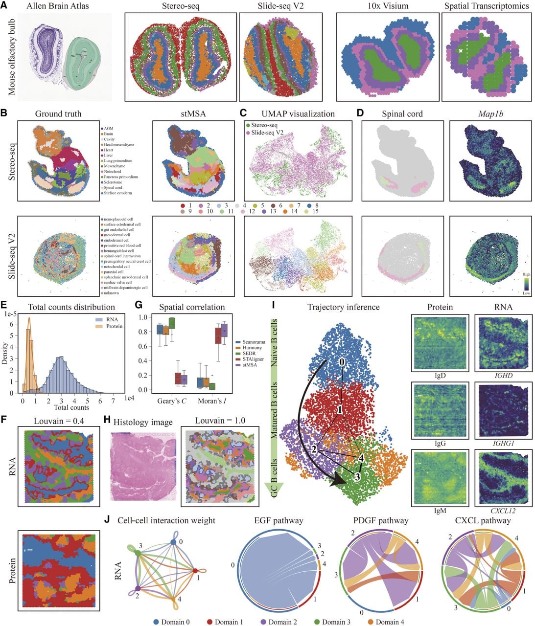
Next, we assessed stMSA's performance with smaller data sets. Specifically, we applied stMSA to two mouse olfactory bulb slices obtained via the 10x Visium and ST (Ståhl et al. 2016) platforms, which contained 918 and 267 spots, respectively. The domain identification results (Fig. 4A; Supplemental Fig. S12A) demonstrated that stMSA was the only method capable of accurately identifying the joint domain structure. In contrast, other methods incorrectly assigned the same domain in different slices while using distinct cluster labels. Additionally, UMAP visualizations (Supplemental Fig. S12B) indicated that stMSA effectively mitigated batch effects across the two sequencing platforms, validating its capability to learn a batch effect–free latent representation even in small-scale data sets. Furthermore, the quantitative integration scores demonstrate stMSA's effectiveness in integrating cross-sequencing techniques and eliminating batch effects (Supplemental Fig. S10B).
Furthermore, we examined stMSA's ability to integrate data from imbalanced data set sizes, as different sequencing platforms may capture data at varying resolutions. To prevent the larger data set from dominating the integration, stMSA randomly assigns cells from the larger data set into several new, independent groups for representation learning, thereby balancing its contribution against the smaller data set. For this evaluation, we utilized embryonic day (E) 9.5 mouse embryo data from the Stereo-seq platform (4356 spots) and the Slide-seq V2 platform (14,758 spots) (Fig. 4B). The results revealed that stMSA effectively integrated the imbalanced slices, producing accurate joint domain identification results (Fig. 4B,C). In contrast, Scanorama, Harmony, SEDR, and CAST exhibited significant batch effects in its latent representation, as shown in the batch UMAP visualization, and STAligner and STAMP struggled to identify joint domains (Supplemental Fig. S13).
To further validate the reliability of stMSA's domain identification results, we compared the spatial distribution of identified domains with the expression patterns of corresponding marker genes, which have been confirmed by previous biological experiments. Notable tissue structures, including the brain, heart, spinal cord, lung, and sclerotome, demonstrated a strong correlation with their respective marker genes: Crabp2 for the brain (Pietilä et al. 2023), Actc1 for the heart (Frank et al. 2019), Map1b for the spinal cord (Tortosa et al. 2011), Ptn for the lung (Weng and Liu 2010), and Pax1 for the sclerotome (Fig. 4D; Supplemental Fig. S14; Dong et al. 2018). These findings further corroborate the accuracy of stMSA in domain identification, demonstrating its applicability across various sequencing platforms and data set sizes.
In conclusion, evaluation through UMAP visualization and quantitative integration scores confirms that stMSA achieves effective elimination of batch effects originating from both experimental protocols and sequencing techniques (Supplemental Fig. S10C).
Deciphering B cell development trajectories through spatial multiomics integration in human tonsils
To explore the integration of spatial proteomics and transcriptomics data, we applied stMSA to a human tonsil data set, utilizing spatial CITE-seq for proteomics and the 10x Visium platform for transcriptomics (Liu et al. 2023). This integration enables a more comprehensive understanding of cellular functions (Lundberg and Borner 2019), particularly for B cell development in the tonsil. Notably, the data sets exhibited significant differences in total count distributions across spots for RNA and protein data set, posing challenges for effective data harmonization (Fig. 4E). We first assessed domain identification accuracy on multiomics spatial slices using our input settings (see Methods) and compared performance with other state-of-the-art methods. STAMP, however, could not be applied to integrate RNA and protein data under our preprocessing pipeline because the input data sets violated its foundational assumption of a gamma-Poisson distribution, which is critical to its statistical model. stMSA successfully identified joint RNA–protein spatial domains (Fig. 4F), demonstrating robust cross-omics integration capabilities. In contrast, CAST failed to harmonize transcriptomic and proteomic slices effectively (Supplemental Fig. S15).
We further evaluated stMSA with methods capable of robust RNA–protein integration (focusing on those demonstrating successful cross-omics alignment). stMSA generated the most expressive latent representations, achieving the lowest Geary's C (minimizing spatial randomness) and highest Moran's I (maximizing spatial dependency) (Fig. 4G). This underscores stMSA's ability to harmonize data patterns from heterogeneous sources in the human tonsil data set.
To enhance domain resolution, we adjusted the Louvain clustering algorithm's resolution parameter to 1.0, enabling finer domain delineation. This adjustment allowed us to clearly identify the lymph follicular region, with the follicular center designated as domain 6 and the extrafollicular plasma cell region as domain 3, aligning well with histological observations (Fig. 4H; Supplemental Fig. S16). Subsequent analysis of spatially variable genes (SVGs) within the follicular region revealed associations with lymph follicular functions (Boyd et al. 2013; Hwang et al. 2013).
Utilizing the latent representation generated by stMSA for trajectory inference, we found that identified domains aligned well with the developmental stages of B cells. Specific marker proteins and genes, such as IgD and IGHD for naive B cells (Espinoza et al. 2023), IgG and IGHG1 for mature B cells (King et al. 2021), and IgM and CXCL12 for germinal center (GC) B cells (Barinov et al. 2017), corroborated this alignment (Fig. 4I). The spatial distribution of these markers closely corresponded with the domains identified by stMSA, showcasing a coherent relationship with B cell development. We also utilized CellChat (Jin et al. 2021) to analyze cell–cell communication based on domain identification results. The analysis revealed significant interactions among domains 2, 3, and 4, whereas domain 0 primarily interacted with domain 1. Notably, domain 1 engaged with all other domains, supporting the inferred B cell development trajectory. Pathway analysis indicated that these interactions were pathway specific: Domain 0 interacted with domain 1 via the EGF pathway, whereas domains 2, 3, and 4 primarily connected through the PDGF and CXCL pathways (Fig. 4J).
We further validated stMSA by integrating mouse spleen transcriptomics (SPOTS) (Ben-Chetrit et al. 2023) and proteomics (spatial CITE-seq) (Liu et al. 2023) data. stMSA successfully harmonized RNA and protein spots in a unified embedding space (Supplemental Fig. S17B), aligning with tissue histology (Supplemental Fig. S17A) to resolve distinct splenic architectures. In summary, the experimental results demonstrate that stMSA is capable of integrating multiomics data effectively. It successfully captures the developmental patterns within the multiomics data sets, accurately identifies domain results, and constructs a correct developmental trajectory of B cells in the human tonsil data set.
Elucidating tissue identity through cross-slice matching in embryonic development
Matching spots across adjacent SO slices is critical for understanding the developmental trajectories of various cell types, tissues, and the process of organogenesis. This matching involves establishing correspondences between spot pairs from different slices taken at varying developmental stages, ensuring that matched spots exhibit similar gene expression profiles while preserving the spatial relationships inherent in each SO slice. To evaluate the cross-slice matching capabilities of stMSA, we applied the model to the Mouse Organogenesis Spatiotemporal Transcriptomic Atlas (MOSTA) data set (Chen et al. 2022).
The results of applying stMSA to match tissue types between two mouse embryo slices collected on E14.5 and E15.5 are illustrated in Figure 5A. The Sankey plot in Figure 5B demonstrates effective matching between these slices, revealing that most tissue types in mature organs, including the brain, heart, muscle, liver, and lung, have been accurately aligned. Furthermore, this matching process enabled us to identify specific organogenesis stages, such as the finding that cartilage at stage E15.5 develops from cartilage and cartilage primordium at stage E14.5. This developmental relationship is supported by the matching results shown in Figure 5C, which highlights only the matched spot pairs between the two tissues. To further validate this relationship, we visualized the spatial distribution of Col2a1, a marker gene for cartilage (Hissnauer et al. 2010), alongside the domain distribution of cartilage and cartilage primordium at stage E14.5. Notably, the expression pattern of Col2a1 aligned closely with the corresponding domain distributions (Fig. 5D).
stMSA demonstrates effective tissue matching abilities in the Mouse Organogenesis Spatiotemporal Transcriptomic Atlas (MOSTA) data set. (A) Visualization of the cross-slice matching results between the E14.5 and E15.5 stages of mouse embryo. To improve the clarity of the matching results, 500 matched spot pairs were randomly selected. (B) The Sankey graph illustrating the tissue matching between the E14.5 and E15.5 stages, with a highlighted path showcasing the matching relation between cartilage and cartilage primordium. (C) Matched spot pairs specifically focusing on the cartilage–cartilage primordium relationship at the E14.5 and E15.5 stages. (D) Marker gene expression patterns and spatial domain distributions of cartilage and cartilage primordium at the E14.5 stage. (E) Confidence scores of the matching results. The confidence scores quantify the accuracy of cross-slice cell type matches, with higher scores reflecting stronger alignment confidence. For each spot, the score is computed as the proportion of matched cell type pairs relative to the total identified pairs (cell type–matched pairs/total pairs). Thus, a higher score indicates greater precision in the biological correspondence for that spot. (F) Comparison of the matching scores between stMSA and SLAT under different settings (RAW, HVG, PCA, and DPCA init).
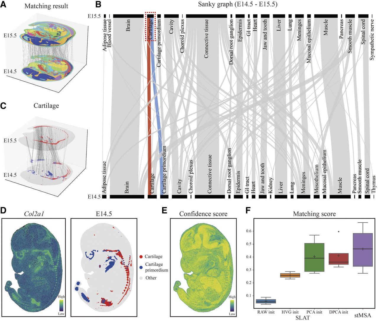
To quantitatively assess the overall matching performance of stMSA, we calculated a confidence score that evaluates the similarity between the embedded spots that were matched. This score, defined as the cosine distance between the embeddings of two matched spots, is presented in Figure 5E for the E14.5 slice, clearly illustrating a high degree of similarity between the matched spots. Additionally, we extended our analysis to examine cross-slice matching between pairs at other stages, specifically E9.5–E10.5, E10.5–E11.5, E11.5–E12.5, E12.5–E13.5, and E13.5–E14.5. We compared the matching results with those obtained using the spatial-linked analysis of transcriptomics (SLAT), which has four different initialization settings based on input types: using all genes (raw init), only highly variable genes (HVG init), dimension-reduced gene expression profiles based on principal component analysis (PCA init), and dual PCA (DPCA init) (Xia et al. 2023). Figure 5F summarizes the matching scores obtained by stMSA and the four SLAT versions (for details, see Supplemental Note S1), demonstrating that stMSA outperforms SLAT across various settings.
stMSA enables multislice spatial alignment
Current sequencing technologies limit researchers to capturing 2D slices of biological tissues, posing challenges in fully understanding 3D biological structures. To address this, stMSA proposed an automated SO alignment through a landmark domain-guided enhanced iterative closest point (ICP) algorithm, which optimizes a rotation matrix for cross-slice coordinate harmonization (see Methods).
We first benchmarked stMSA against leading alignment tools PASTE (Zeira et al. 2022), STAligner (Zhou et al. 2023), and SANTO (Li et al. 2024) using a two-slice mouse spleen ST data set (Ben-Chetrit et al. 2023). The initial positioning of these two slices exhibits a substantial spatial misalignment, necessitating further refinement to achieve precise alignment (Fig. 6A). stMSA leveraged the macrophage-enriched (MP-enriched) region as the landmark domain to guide alignment, validated by the spatial distribution of the macrophage-associated gene marker Rsad2 (Supplemental Fig. S18A; Ding et al. 2025). Visual assessment confirmed stMSA's accuracy in reconstructing coherent 3D tissue structures from 2D slices (Fig. 6B), whereas PASTE achieved only partial alignment, and STAligner/SANTO failed to establish spatial correspondence. Quantitatively, stMSA outperformed all competing methods, achieving the highest Pearson correlation coefficient (PCC) and cell type matching index (CI) scores (Fig. 6C).
The alignment performance of stMSA on multislice SO data sets. (A) Original unaligned 2D/3D spatial coordinates from the mouse spleen data set. (B) Comparative visualization of alignment results from stMSA and three benchmark methods on the mouse spleen data set. (C) Quantitative evaluation of alignment performance using PCC and CI scores. Error bars represent the 95% confidence intervals of the PCC and CI scores. (D) Alignment robustness assessment across different anatomical orientations (coronal sections) of the mouse brain, measured by PCC and CI. (E) 3D reconstruction of original (left) and stMSA-aligned (right) spatial coordinates, demonstrating accurate spatial preservation. (F) Original coronal mouse brain orientation, stMSA-derived spatial domains, and pyramidal cell layer marker gene spatial distribution.
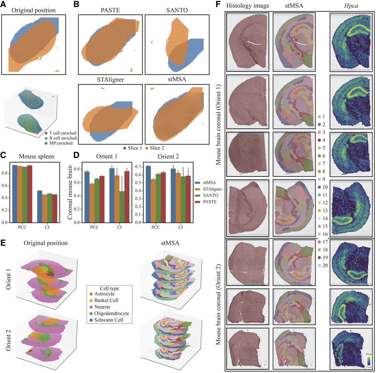
To assess scalability, we applied stMSA to align seven coronal sections from mouse brains (Ballester Roig et al. 2023). This data set contained two flipped orientations, including “orient 1” (four slices) and “orient 2” (three slices), with significant initial misalignment (Fig. 6E, left). stMSA first identified spatial domains consistent with the Allen Brain Atlas annotations (Fig. 3F). For instance, the pyramidal layer (domain 7) in the hippocampus aligned precisely with both the histology-derived hook-like structure and the expression pattern of the marker gene Hpca (Tzingounis et al. 2007), prompting its selection as the landmark domain for alignment.
Using a modified ICP algorithm, stMSA successfully reconciled rotations and flips between “orient 1” and “orient 2,” integrating all slices into a unified coordinate system (Fig. 6E, right). Quantitative evaluation confirmed stMSA's superior alignment scores for both orientations (Fig. 6D), with 2D visualizations further validating coherent integration (Supplemental Fig. S18B). Together, these results demonstrate stMSA's robustness in aligning multiple SO slices, enabling accurate 3D tissue reconstruction.
Discussion
The rapid advancement of sequencing technologies has resulted in the generation of an increasing volume of high-quality SO data. This growth has created a pressing need to integrate SO data from diverse sources, which may vary in experimental protocols, sequencing platforms, size, shape, and orientation. In this work, we present a novel contrastive learning–based method, termed stMSA, designed for the integration of multiple SO data sets. stMSA learns cross-batch spot embeddings by optimizing two key principles: (1) enhancing the similarity of embeddings within a slice for spots situated in connected spatial niches and (2) maximizing the similarity of embeddings between cross-batch spots with analogous gene expression profiles. By adhering to these principles, stMSA effectively captures the distribution patterns of spots both within and across slices. Additionally, stMSA employs graph attention–based autoencoder techniques and DEC to optimize model parameters and reconstruct gene expression profiles.
stMSA preserves slice-specific biological signals and prevents overmixing through two complementary approaches. The framework first employs GER to constrain the model to reproduce original transcriptional patterns, ensuring conservation of unique biological signatures. Simultaneously, it only identifies high-confidence cross-slice similarity pairs (MNNs) using dynamic stringent thresholding, thereby mitigating overmixing between different slices. These two strategies prioritize biologically conserved features while maintaining distinct slice-specific profiles, effectively balancing data harmonization with biological fidelity.
A key advantage of stMSA lies in its ability to integrate multiple SO slices, thereby overcoming the limitations of single-slice analysis. Traditional single-slice approaches often produce fragmented or misaligned spatial domains, particularly in tissues with structural continuity. In contrast, stMSA jointly analyzes adjacent sections to yield consistent and biologically meaningful domain identification across slices, eliminating the need for manual correction. Moreover, stMSA projects multislice data into a unified latent space, enabling downstream analyses in a pseudo-3D context. This approach facilitates tasks such as reconstructing cross-slice developmental trajectories and aligning multiple unaligned spatial slices. These capabilities allow stMSA to uncover spatially conserved biological processes and microenvironments that are typically inaccessible through isolated single-slice analyses.
Although stMSA demonstrates robust performance in SO integration, we acknowledge that its current implementation has higher computational demands compared with state-of-the-art tools. For example, when aligning 20 consecutive slices (4226 spots per slice), stMSA requires ∼15 min and 12 GB of GPU memory. Under identical hardware conditions, CAST completes the alignment in ∼8 min using 14 GB GPU memory, whereas STAMP requires ∼32 min with only 1 GB GPU memory (Supplemental Fig. S4). This mainly stems from stMSA's multitask optimization architecture; although it enhances model performance, it results in higher computational costs. In future work, we will prioritize algorithmic optimizations to reduce the model's runtime and memory consumption while retaining its performance.
In conclusion, our results demonstrate that stMSA offers a comprehensive solution for integrating multiple SO slices from different sources, facilitating integrative analyses of SO data. We strongly believe that as SO sequencing technologies continue to evolve, stMSA will further empower researchers to uncover novel biological insights from an increasingly diverse array of SO data sets.
Methods
Data preprocessing
To prepare the data for analysis, the raw gene expressions undergo an initial log transformation and normalization using the Python package SCANPY (Wolf et al. 2018). To overcome the zero inflation in ST data, stMSA selects the top k highly variable genes (HVGs) as input features. For SO slices with common gene backgrounds, such as the DLPFC data set (Maynard et al. 2021), we set k as 3000 by default. For SO slices with varying genes, usually derived from different platforms, it is suggested to set k higher and use the intersecting genes as input features. For proteomics and transcriptomics integration, we use the principal component analysis (PCA) (Jolliffe and Cadima 2016) to decompose the protein and RNA data and use the top 300 principal components (PCs) as the input features.
Spatial graph construction for SO slices
We first construct a spatial graph for each slice based on the spot coordinates. Given the spot coordinates on slice t, represented as st, we denote the spatial information of all k slices as set S = {s1, s2, …, sk}. stMSA initially calculates the Euclidean distances between all spots within each slice. Then, stMSA uses a radius threshold r to define the edges between spots. We fine-tuned the radius threshold r to achieve spatial graphs with an approximate connectivity of six neighbors for each spot by default. The adjacency matrices for spatial graphs are denoted as , where is set as one only if spot i and spot j within slice st are connected, and it is assigned zero otherwise. For the imbalanced data sets, we randomly sampled the large slice into two small data sets and treated them as two individual slices.
Representation learning via parameter-shared graph auto-encoder
To effectively couple gene expression and spatial information, stMSA uses the technique of parameter-shared graph autoencoder to learn the latent embeddings of spots. Specifically, the graph auto-encoder consists of a graph attention network (GAT) (Veličković et al. 2018) and a fully connected network (FCN) (Yosinski et al. 2015) for both the encoder and the decoder. Furthermore, to facilitate model convergence, stMSA shares the GAT and FCN parameters between the encoder and the decoder.
Encoder
stMSA adopts the GAT network to aggregate spot features within a local spatial niche on a slice. In contrast to graph convolutional neural networks, GAT uses the self-attention mechanism to dynamically compute the importance of inter-spot connections during the feature aggregation process. Specifically, the GAT layer takes the gene expression profiles and the spatial graph of each slice as inputs. Suppose the gene expression profiles on slice sm are denoted as , where indicates the gene expression of spot i, and denotes the number of spots in slice sm; the formulation of the GAT layer is described as follows:
Subsequently, stMSA employs a FCN further to compress the initial latent embedding into a lower dimension as shown in the following equation:
Decoder
The decoder in stMSA also consists of a GAT layer and an FCN layer, both designed to reconstruct the input gene expressions. To expedite convergence and enhance efficiency, the decoder layers share the parameters learned from the encoder layers. Specifically, stMSA utilizes the transposed weight matrix of the encoder as the weight matrix for the corresponding decoder layers. Additionally, it directly incorporates the attention coefficients from the encoder's GAT layer into the decoder's GAT layer. The formula for the decoder is as follows:
Enhancing multislice integration via graph contrastive learning
To create a unified embedding space for spot features extracted from various slices, stMSA employs a contrastive learning approach to remove batch effects while preserving the original spatial patterns of the spots. In contrast to conventional graph contrastive learning methods that require building a corrupted graph, our approach leverages spatial graphs constructed from multiple input SO slices. It consists of two components: inner-batch contrastive learning and cross-batch contrastive learning.
Inner-batch contrastive learning
In the inner-batch contrastive learning stage, the model is constrained to generate embeddings that closely resemble those of adjacent spots and separate those nonadjacent spots. To achieve this, stMSA maximizes the embedding similarity between a centroid spot i and a spot in its adjacent spatial niche (denoted as positive pairs), while minimizing its similarity with a randomly sampled spot k (denoted as negative pairs) within the same batch (i.e., slice), and this process is formulated as follows:
Cross-batch pair identification
stMSA initiates cross-batch contrastive learning by dynamically selecting and refining cross-slice similar pairs. For each two distinct slices from all input slices, stMSA identifies candidate similar pairs by computing the L2 distance between spot embeddings, selecting the k-nearest neighbors (k-NNs) for each spot. To ensure high-confidence matches, pairs with L2 distances >75% of the maximum distance are filtered out, whereas only pairs with distances below this threshold are retained. Retained pairs are further refined by retaining only MNNs in which spots reciprocally rank in each other's k-NN lists to minimize spurious associations. These curated MNNs serve as positive pairs to maximize similarity during cross-batch contrastive learning.
To adapt to evolving embeddings, cross-batch pairs are regenerated every 100 epochs. During initial training (epoch 0), embeddings are derived from the top 30 PCs of the input data, enabling stable cold-start optimization.
Cross-batch contrastive learning
In the cross-batch contrastive learning stage, stMSA aims to generate batch-corrected embedding for each spot, which also reserves the spatial gene expression pattern. To achieve this, stMSA maximizes the embedding similarity between the centroid spot i and a spot j with similar gene expression in another slice (denoted as positive pairs), while simultaneously minimizing the similarity with a randomly sampled spot k (denoted as negative pairs) across slices. This process is depicted as follows:
The objective function of the two contrastive learning stages can be expressed as follows:
Because of the large number of spots in each batch and the relatively low neighbor count that we have set, the probability of sampling nearby spots in randomly selected negative pairs is extremely low. This ensures that the model can effectively discriminate the similarities and differences among spots. Additionally, incorporating the minimization of similarity between negative pairs helps prevent a scenario in which the embeddings of all spots become excessively similar, which will affect the performance of downstream tasks.
GER via graph autoencoder
The goal of GER is to generate embeddings that can capture unique gene expression patterns, preserving their inherent characteristics while avoiding excessive similarity to neighboring spots. To accomplish this, the objective is to maximize the similarity between the input gene expression and the reconstructed output. The loss function is expressed as follows:
Domain distribution tuning with DEC
The domain distribution tuning (DDT) task aims to refine the clustering performance using the DEC technique (Xie et al. 2016). The primary goal is to minimize the distance between the soft clustering distribution (Krizhevsky et al. 2017) and the auxiliary target distribution, as depicted below:
In sum, the overall loss function is defined as follows:
In all experiments conducted in this study, we set the loss weights to 1.0 for both the contrastive learning and GER loss and to 0.01 for the DDT loss. This weighting scheme emerged from empirical validation across diverse data sets, demonstrating effective balance between objectives while maintaining robust task performance in our evaluations. Although these fixed parameters delivered consistent results across all tested conditions, users working with their own data types may optionally adjust these weights to prioritize specific tasks.
Moreover, we conducted an ablation study to assess the individual contributions of each loss function (Supplemental Note S3.1), quantifying their impact on spatial integration performance.
Joint domain detection across SO slices
After encoding the spot features across different SO slices into a coherent embedding space, we use the unsupervised clustering technique to identify the spatial domains in the joint embedding space. For data sets with known labels or prior knowledge of the cluster number, stMSA employs the finite Gaussian mixture clustering model from the R package MCLUST (Scrucca et al. 2016) to identify spatial domains. In cases in which the cluster number is unknown, stMSA utilizes the Louvain clustering algorithm for community detection (Blondel et al. 2008), which has been implemented in the Python package SCANPY (Wolf et al. 2018).
Cross-slice matching
The objective of matching spots across two adjacent SO slices is to establish a mapping between pairs of spots from different slices, ensuring that the matched spots exhibit similar gene expression patterns. Additionally, the mapping should preserve the spatial relationship of spots within each SO slice. To achieve this, we calculate the Euclidean distances in the embedding space between each spot s on the source slice and all other spots on the target slice. The spot t on the target slice with the smallest Euclidean distance to spot s is considered its match.
Multislice alignment
Aligning multislice data is a key step in reconstructing 2D tissue slices into 3D. In this regard, stMSA incorporates landmark points to guide the alignment process. Given the absence of dedicated SO alignment methods, we have enhanced the iterative closest point (ICP) algorithm (Besl and McKay 1992) to align slices using the domain detection output from stMSA.
ICP with disturbance
The alignment procedure employed in stMSA comprises three primary components: (1) integration of multislice data using stMSA, (2) identification of the landmark domain, and (3) derivation of the transformation matrix through a modified version of the ICP algorithm.
The ICP algorithm is renowned for its efficiency and simplicity, making it one of the most extensively utilized point cloud registration methods. The objective function for the ICP alignment is stated as follows:
Given the nonconvex nature of the problem and the dependency on local iterative steps, the ICP algorithm is prone to converging to local minima (Yang et al. 2016). To address this concern, stMSA incorporates a threshold, in which the mean error between two iterations should be below the threshold to halt the iteration process. If the threshold is surpassed, the point cloud undergoes rotation and the iteration persists. Empirically, this strategy effectively enables ICP to avoid local minima (Supplemental Note S3.2).
The overall structure of stMSA
The dimensions of the layers in the auto-encoder are set as follows: The input data shape is 512 in the encoder GAT layer and is 512 to 30 in the encoder FCN layer. The decoder is symmetric to the encoder. To optimize the model parameters, we use the Adam optimizer (Kingma and Ba 2017) with a learning rate of 0.001. We implement the stMSA model using the popular graph neural network framework PyTorch Geometric (PyG) (Fey and Lenssen 2019). We set the number of training epochs to 500. In the cross-batch contrastive learning, we update the cross-batch pairs, and for the DDT task, we update the DEC p distribution every 100 epochs.
Evaluation metrics
The descriptions of all evaluation metrics applied in this study are detailed in Supplemental Note S4.
Data sets
Multiple SO data sets derived from human and mouse tissues, organs, and embryos are used to evaluate the performance of stMSA. Specifically, the DLPFC data set can be obtained from the Lieber Institute GitHub repository at https://github.com/LieberInstitute/HumanPilot. The Stereo-seq DLPFC data set can be found at NGDC database (https://ngdc.cncb.ac.cn/?lang=en) BioProject PRJCA009779. The mouse brain serial data set can be accessed at STOmicsDB (anterior: https://db.cngb.org/stomics/datasets/STDS0000018; posterior: https://db.cngb.org/stomics/datasets/STDS0000021). The mouse brain coronal fresh-frozen H&E and DAPI (IF) stained data set can be found at squidpy data set (H&E: https://squidpy.readthedocs.io/en/stable/api/squidpy.datasets.visium_hne_adata.html; DAPI: https://squidpy.readthedocs.io/en/stable/api/squidpy.datasets.visium_fluo_adata.html). The mouse brain coronal FFPE data set can be found at STOmicsDB (https://db.cngb.org/stomics/datasets/STDS0000052). The FF and FFPE mouse brain data set can be found at the 10x Genomics database (FF: https://www.10xgenomics.com/datasets/adult-mouse-brain-coronal-section-visium-ff-1-standard; FFPE: https://www.10xgenomics.com/datasets/mouse-brain-coronal-section-1-ffpe-2-standard). The Slide-seq V2 mouse brain bulb data can be obtained from the Broad Institute webpage (https://singlecell.broadinstitute.org/single_cell/study/SCP815/highly-sensitive-spatial-transcriptomics-at-near-cellular-resolution-with-slide-seqv2#study-download). The Stereo-seq mouse olfactory bulb data set can be accessed from the SEDR GitHub repository (https://github.com/JinmiaoChenLab/SEDR_analyses/tree/master/data). The Visium mouse olfactory bulb data can be found at the NCBI Gene Expression Omnibus (GEO; https://www.ncbi.nlm.nih.gov/geo/) under accession number GSM4656181. The ST mouse olfactory bulb can be found at the NCBI BioProject database (https://www.ncbi.nlm.nih.gov/bioproject/) under accession number PRJNA316587. The MOSTA data set can be found at STOmicsDB (https://db.cngb.org/stomics/mosta/spatial/). The Slide-seq V2 mouse embryo data set can be found at the CELLxGENE database (https://datasets.cellxgene.cziscience.com/acc80ff4-5dee-46cc-bf22-84a9a83c9c38.h5ad). The proteomics human tonsil and mouse spleen data set can be found at GEO under accession number GSE213264. The 10x Visium human tonsil data set can be found at the 10x Genomics database (https://www.10xgenomics.com/datasets/visium-cytassist-gene-and-protein-expression-library-of-human-tonsil-with-add-on-antibodies-h-e-6-5-mm-ffpe-2-standard). The mouse spleen ST data set can be found under GEO accession number GSE198353. The mouse brain coronal data set can be found at STOmicsDB (https://db.cngb.org/stomics/datasets/STDS0000218).
A summary of the data set information can be found in Supplemental Tables S1 and S2.
Software availability
The implemented code is available at GitHub (https://github.com/hannshu/stMSA) and as Supplemental Code.
Competing interest statement
The authors declare no competing interests.
Acknowledgments
We thank all the contributors of the open-source data sets and freely available tools used in this study. We also appreciate the reviewer suggestions. This work has been supported by the National Natural Science Foundation of China (grant no. 62402382) and the Natural Science Project of Shaanxi Provincial Department of Education (grant no. 23JK0562).
Author contributions: T.W., J.C., Q.J., and X.S. conceived the study and experiments; H.S. implemented the software and conducted the analyses; H.S., C.X., J.H., Y.W., and J.P. analyzed the results; T.W., J.C., H.S, and C.X. wrote and reviewed the manuscript; and X.S., T.W., and J.P. supervised the research and provided funding support.
Notes
[1] Supplementary material [Supplemental material is available for this article.]
[2] Article published online before print. Article, supplemental material, and publication date are at https://www.genome.org/cgi/doi/10.1101/gr.280584.125.
References
- ↵Asp M, Bergenstråhle J, Lundeberg J. 2020. Spatially resolved transcriptomes: next generation tools for tissue exploration. Bioessays 42: 1900221. 10.1002/bies.201900221
- ↵Ballester Roig MN, Leduc T, Dufort-Gervais J, Maghmoul Y, Tastet O, Mongrain V. 2023. Probing pathways by which rhynchophylline modifies sleep using spatial transcriptomics. Biol Direct 18: 21. 10.1186/s13062-023-00377-7
- ↵Barinov A, Luo L, Gasse P, Meas-Yedid V, Donnadieu E, Arenzana-Seisdedos F, Vieira P. 2017. Essential role of immobilized chemokine CXCL12 in the regulation of the humoral immune response. Proc Natl Acad Sci 114: 2319–2324. 10.1073/pnas.1611958114
- ↵Ben-Chetrit N, Niu X, Swett AD, Sotelo J, Jiao MS, Stewart CM, Potenski C, Mielinis P, Roelli P, Stoeckius M, 2023. Integration of whole transcriptome spatial profiling with protein markers. Nat Biotechnol 41: 788–793. 10.1038/s41587-022-01536-3
- ↵Besl P, McKay ND. 1992. A method for registration of 3-D shapes. IEEE Trans Pattern Anal Mach Intell 14: 239–256. 10.1109/34.121791
- ↵Blondel VD, Guillaume JL, Lambiotte R, Lefebvre E. 2008. Fast unfolding of communities in large networks. J Stat Mech 2008: P10008. 10.1088/1742-5468/2008/10/P10008
- ↵Boyd SD, Natkunam Y, Allen JR, Warnke RA. 2013. Selective immunophenotyping for diagnosis of B-cell neoplasms: immunohistochemistry and flow cytometry strategies and results. Appl Immunohistochem Mol Morphol 21: 116–131. 10.1097/PAI.0b013e31825d550a
- ↵Chen A, Liao S, Cheng M, Ma K, Wu L, Lai Y, Qiu X, Yang J, Xu J, Hao S, 2022. Spatiotemporal transcriptomic atlas of mouse organogenesis using DNA nanoball-patterned arrays. Cell 185: 1777–1792.e21. 10.1016/j.cell.2022.04.003
- ↵Cheng M, Jiang Y, Xu J, Mentis AFA, Wang S, Zheng H, Sahu SK, Liu L, Xu X. 2023. Spatially resolved transcriptomics: a comprehensive review of their technological advances, applications, and challenges. J Genet Genomics 50: 625–640. 10.1016/j.jgg.2023.03.011
- ↵Clevert DA, Unterthiner T, Hochreiter S. 2016. Fast and accurate deep network learning by exponential linear units (ELUs). arXiv:1511.07289 [cs.LG]. 10.48550/arxiv.1511.07289
- ↵Ding X, Zhou Y, Qiu X, Xu X, Hu X, Qin J, Chen Y, Zhang M, Ke J, Liu Z, 2025. RSAD2: a pathogenic interferon-stimulated gene at the maternal-fetal interface of patients with systemic lupus erythematosus. Cell Rep Med 6: 101974. 10.1016/j.xcrm.2025.101974
- ↵Dong K, Zhang S. 2022. Deciphering spatial domains from spatially resolved transcriptomics with an adaptive graph attention auto-encoder. Nat Commun 13: 1739. 10.1038/s41467-022-29439-6
- ↵Dong J, Hu Y, Fan X, Wu X, Mao Y, Hu B, Guo H, Wen L, Tang F. 2018. Single-cell RNA-seq analysis unveils a prevalent epithelial/mesenchymal hybrid state during mouse organogenesis. Genome Biol 19: 31. 10.1186/s13059-018-1416-2
- ↵Espinoza DA, Coz CL, Cabrera EC, Romberg N, Bar-Or A, Li R. 2023. Distinct stage-specific transcriptional states of B cells derived from human tonsillar tissue. JCI Insight 8: e155199. 10.1172/jci.insight.155199
- ↵Fey M, Lenssen JE. 2019. Fast graph representation learning with PyTorch Geometric. arXiv:1903.02428 [cs.LG]. 10.48550/arxiv.1903.02428
- ↵Frank D, Rangrez AY, Friedrich C, Dittmann S, Stallmeyer B, Yadav P, Bernt A, Schulze-Bahr E, Borlepawar A, Zimmermann W-H, 2019. Cardiac α-actin (ACTC1) gene mutation causes atrial-septal defects associated with late-onset dilated cardiomyopathy. Circ Genom Precis Med 12: e002491. 10.1161/CIRCGEN.119.002491
- ↵Fulcher BD, Murray JD, Zerbi V, Wang XJ. 2019. Multimodal gradients across mouse cortex. Proc Natl Acad Sci 116: 4689–4695. 10.1073/pnas.1814144116
- ↵Grimstvedt JS, Shelton AM, Hoerder-Suabedissen A, Oliver DK, Berndtsson CH, Blankvoort S, Nair RR, Packer AM, Witter MP, Kentros CG. 2023. A multifaceted architectural framework of the mouse claustrum complex. J Comp Neurol 531: 1772–1795. 10.1002/cne.25539
- ↵Hie B, Bryson B, Berger B. 2019. Efficient integration of heterogeneous single-cell transcriptomes using Scanorama. Nat Biotechnol 37: 685–691. 10.1038/s41587-019-0113-3
- ↵Hissnauer TN, Baranowsky A, Pestka JM, Streichert T, Wiegandt K, Goepfert C, Beil FT, Albers J, Schulze J, Ueblacker P, 2010. Identification of molecular markers for articular cartilage. Osteoarthritis Cartilage 18: 1630–1638. 10.1016/j.joca.2010.10.002
- ↵Hoerder-Suabedissen A, Ocana-Santero G, Draper TH, Scott SA, Kimani JG, Shelton AM, Butt SJB, Molnár Z, Packer AM. 2023. Temporal origin of mouse claustrum and development of its cortical projections. Cereb Cortex 33: 3944–3959. 10.1093/cercor/bhac318
- ↵Hwang IY, Hwang KS, Park C, Harrison KA, Kehrl JH. 2013. Rgs13 constrains early B cell responses and limits germinal center sizes. PLoS One 8: e60139. 10.1371/journal.pone.0060139
- ↵Jin S, Guerrero-Juarez CF, Zhang L, Chang I, Ramos R, Kuan CH, Myung P, Plikus MV, Nie Q. 2021. Inference and analysis of cell-cell communication using CellChat. Nat Commun 12: 1088. 10.1038/s41467-021-21246-9
- ↵Jolliffe IT, Cadima J. 2016. Principal component analysis: a review and recent developments. Philos Trans A Math Phys Eng Sci 374: 20150202. 10.1098/rsta.2015.0202
- ↵King HW, Orban N, Riches JC, Clear AJ, Warnes G, Teichmann SA, James LK. 2021. Single-cell analysis of human B cell maturation predicts how antibody class switching shapes selection dynamics. Sci Immunol 6: eabe6291. 10.1126/sciimmunol.abe6291
- ↵Kingma DP, Ba J. 2017. Adam: a method for stochastic optimization. arXiv:1412.6980 [cs.LG]. 10.48550/arxiv.1412.6980
- ↵Korsunsky I, Millard N, Fan J, Slowikowski K, Zhang F, Wei K, Baglaenko Y, Brenner M, Loh PR, Raychaudhuri S. 2019. Fast, sensitive and accurate integration of single-cell data with harmony. Nat Methods 16: 1289–1296. 10.1038/s41592-019-0619-0
- ↵Krizhevsky A, Sutskever I, Hinton GE. 2017. ImageNet classification with deep convolutional neural networks. Commun ACM 60: 84–90. 10.1145/3065386
- ↵Li J, Chen S, Pan X, Yuan Y, Shen HB. 2022. Cell clustering for spatial transcriptomics data with graph neural networks. Nat Comput Sci 2: 399–408. 10.1038/s43588-022-00266-5
- ↵Li H, Lin Y, He W, Han W, Xu X, Xu C, Gao E, Zhao H, Gao X. 2024. SANTO: a coarse-to-fine alignment and stitching method for spatial omics. Nat Commun 15: 6048. 10.1038/s41467-024-50308-x
- ↵Liu Y, DiStasio M, Su G, Asashima H, Enninful A, Qin X, Deng Y, Nam J, Gao F, Bordignon P, 2023. High-plex protein and whole transcriptome co-mapping at cellular resolution with spatial CITE-seq. Nat Biotechnol 41: 1405–1409. 10.1038/s41587-023-01676-0
- ↵Lundberg E, Borner GHH. 2019. Spatial proteomics: a powerful discovery tool for cell biology. Nat Rev Mol Cell Biol 20: 285–302. 10.1038/s41580-018-0094-y
- ↵Maynard KR, Collado-Torres L, Weber LM, Uytingco C, Barry BK, Williams SR, Catallini JL, Tran MN, Besich Z, Tippani M, 2021. Transcriptome-scale spatial gene expression in the human dorsolateral prefrontal cortex. Nat Neurosci 24: 425–436. 10.1038/s41593-020-00787-0
- ↵Pietilä R, Del Gaudio F, He L, Vázquez-Liébanas E, Vanlandewijck M, Muhl L, Mocci G, Bjørnholm KD, Lindblad C, Fletcher-Sandersjöö A, 2023. Molecular anatomy of adult mouse leptomeninges. Neuron 111: 3745–3764.e7. 10.1016/j.neuron.2023.09.002
- ↵Sandebring-Matton A, Axenhus M, Bogdanovic N, Winblad B, Schedin-Weiss S, Nilsson P, Tjernberg LO. 2021. Microdissected pyramidal cell proteomics of Alzheimer brain reveals alterations in creatine kinase B-type, 14-3-3-gamma, and heat shock cognate 71. Front Aging Neurosci 13: 735334. 10.3389/fnagi.2021.735334
- ↵Schott M, León-Periñán D, Splendiani E, Strenger L, Licha JR, Pentimalli TM, Schallenberg S, Alles J, Samut Tagliaferro S, Boltengagen A, 2024. Open-ST: high-resolution spatial transcriptomics in 3D. Cell 187: 3953–3972.e26. 10.1016/j.cell.2024.05.055
- ↵Scrucca L, Fop M, Murphy TB, Raftery AE. 2016. mclust 5: clustering, classification and density estimation using Gaussian finite mixture models. R J 8: 289–317. 10.32614/RJ-2016-021
- ↵Ståhl PL, Salmén F, Vickovic S, Lundmark A, Navarro JF, Magnusson J, Giacomello S, Asp M, Westholm JO, Huss M, 2016. Visualization and analysis of gene expression in tissue sections by spatial transcriptomics. Science 353: 78–82. 10.1126/science.aaf2403
- ↵Stickels RR, Murray E, Kumar P, Li J, Marshall JL, Di Bella DJ, Arlotta P, Macosko EZ, Chen F. 2021. Highly sensitive spatial transcriptomics at near-cellular resolution with slide-seqV2. Nat Biotechnol 39: 313–319. 10.1038/s41587-020-0739-1
- ↵Sullivan KE, Kraus L, Kapustina M, Wang L, Stach TR, Lemire AL, Clements J, Cembrowski MS. 2023. Sharp cell-type-identity changes differentiate the retrosplenial cortex from the neocortex. Cell Rep 42: 112206. 10.1016/j.celrep.2023.112206
- ↵Tang Z, Luo S, Zeng H, Huang J, Sui X, Wu M, Wang X. 2024. Search and match across spatial omics samples at single-cell resolution. Nat Methods 21: 1818–1829. 10.1038/s41592-024-02410-7
- ↵Tortosa E, Montenegro-Venegas C, Benoist M, Härtel S, González-Billault C, Esteban JA, Avila J. 2011. Microtubule-associated protein 1B (MAP1B) is required for dendritic spine development and synaptic maturation. J Biol Chem 286: 40638–40648. 10.1074/jbc.M111.271320
- ↵Tzingounis AV, Kobayashi M, Takamatsu K, Nicoll RA. 2007. Hippocalcin gates the calcium activation of the slow afterhyperpolarization in hippocampal pyramidal cells. Neuron 53: 487–493. 10.1016/j.neuron.2007.01.011
- ↵Veličković P, Cucurull G, Casanova A, Romero A, Lio P, Bengio Y. 2018. Graph attention networks. arXiv:1710.10903 [stat.ML]. 10.48550/arxiv.1710.10903
- ↵Wang G, Zhao J, Yan Y, Wang Y, Wu AR, Yang C. 2023. Construction of a 3D whole organism spatial atlas by joint modelling of multiple slices with deep neural networks. Nat Mach Intell 5: 1200–1213. 10.1038/s42256-023-00734-1
- ↵Wei X, Fu S, Li H, Liu Y, Wang S, Feng W, Yang Y, Liu X, Zeng Y-Y, Cheng M, 2022. Single-cell stereo-seq reveals induced progenitor cells involved in axolotl brain regeneration. Science 377: eabp9444. 10.1126/science.abp9444
- ↵Wei S, Luo M, Wang P, Chen R, Jin X, Xu C, Li C, Lin X, Xu Z, Liu H, 2025. Charting the spatial transcriptome of the human cerebral cortex at single-cell resolution. Nat Commun 16: 7702. 10.1038/s41467-025-62793-9
- ↵Weng T, Liu L. 2010. The role of pleiotrophin and β-catenin in fetal lung development. Respir Res 11: 80. 10.1186/1465-9921-11-80
- ↵Williams CG, Lee HJ, Asatsuma T, Vento-Tormo R, Haque A. 2022. An introduction to spatial transcriptomics for biomedical research. Genome Med 14: 68. 10.1186/s13073-022-01075-1
- ↵Wolf FA, Angerer P, Theis FJ. 2018. SCANPY: large-scale single-cell gene expression data analysis. Genome Biol 19: 15. 10.1186/s13059-017-1382-0
- ↵Wolf FA, Hamey FK, Plass M, Solana J, Dahlin JS, Göttgens B, Rajewsky N, Simon L, Theis FJ. 2019. PAGA: graph abstraction reconciles clustering with trajectory inference through a topology preserving map of single cells. Genome Biol 20: 59. 10.1186/s13059-019-1663-x
- ↵Xia CR, Cao ZJ, Tu XM, Gao G. 2023. Spatial-linked alignment tool (SLAT) for aligning heterogenous slices. Nat Commun 14: 7236. 10.1038/s41467-023-43105-5
- ↵Xie J, Girshick R, Farhadi A. 2016. Unsupervised deep embedding for clustering analysis. arXiv:1511.06335 [cs.LG]. 10.48550/arxiv.1511.06335
- ↵Xu H, Wang S, Fang M, Luo S, Chen C, Wan S, Wang R, Tang M, Xue T, Li B, 2023. SPACEL: deep learning-based characterization of spatial transcriptome architectures. Nat Commun 14: 7603. 10.1038/s41467-023-43220-3
- ↵Xu H, Fu H, Long Y, Ang KS, Sethi R, Chong K, Li M, Uddamvathanak R, Lee HK, Ling J, 2024. Unsupervised spatially embedded deep representation of spatial transcriptomics. Genome Med 16: 12. 10.1186/s13073-024-01283-x
- ↵Yang J, Li H, Campbell D, Jia Y. 2016. Go-ICP: a globally optimal solution to 3D ICP point-set registration. IEEE Trans Pattern Anal Mach Intell 38: 2241–2254. 10.1109/TPAMI.2015.2513405
- ↵Yosinski J, Clune J, Nguyen A, Fuchs T, Lipson H. 2015. Understanding neural networks through deep visualization. arXiv:1506.06579 [cs.CV]. 10.48550/arxiv.1506.06579
- ↵Yue L, Liu F, Hu J, Yang P, Wang Y, Dong J, Shu W, Huang X, Wang S. 2023. A guidebook of spatial transcriptomic technologies, data resources and analysis approaches. Comput Struct Biotechnol J 21: 940–955. 10.1016/j.csbj.2023.01.016
- ↵Zeira R, Land M, Strzalkowski A, Raphael BJ. 2022. Alignment and integration of spatial transcriptomics data. Nat Methods 19: 567–575. 10.1038/s41592-022-01459-6
- ↵Zhong C, Ang KS, Chen J. 2024. Interpretable spatially aware dimension reduction of spatial transcriptomics with STAMP. Nat Methods 21: 2072–2083. 10.1038/s41592-024-02463-8
- ↵Zhou X, Dong K, Zhang S. 2023. Integrating spatial transcriptomics data across different conditions, technologies and developmental stages. Nat Comput Sci 3: 894–906. 10.1038/s43588-023-00528-w