Flexible and scalable inference of spatially varying correlation in spatial transcriptomics with spCorr

Chenxin Flora Jiang; Yuxin Yin; Paul Robson; Yuanhao James Li; Jingyi Jessica Li; Dongyuan Song

doi:10.1101/gr.281559.125

Abstract

Spatial transcriptomics has transformed our ability to explore gene expression within its tissue context, enabling us to dissect subtle yet biologically significant variations in situ. Although numerous computational methods have been proposed to identify Spatially Varying Genes (SVGs) by modeling their expression separately, much less effort has been devoted to understanding how correlations between genes change across space. Such Spatially Varying Correlations (SVCs) are critical for understanding biological processes such as gene regulatory mechanisms shaped by local tissue environments, yet existing tools remain limited for this task. To address this gap, we present spCorr, a flexible and scalable regression framework for studying SVCs. spCorr provides interpretable, spot-level estimates of gene correlation and detects gene pairs whose correlations vary across locations or between tissue domains. Through extensive simulations and real-data analyses, we show that spCorr achieves high detection power, reliably controls the False Discovery Rate (FDR), and is computationally efficient. Importantly, spCorr reveals biologically meaningful correlation patterns that highlight fine-scale tissue structures, gene module functions, and region-specific interactions, offering new opportunities to study coordinated gene regulation in spatial transcriptomics.

Understanding how genes coordinate their activity across biological contexts has led to rich insights into biological processes and disease mechanisms. Genes do not function in isolation; instead, genes operate within coordinated networks that dynamically adapt across tissues, spatial locations, developmental stages, environmental conditions, and disease states (Karlebach and Shamir 2008; Yang et al. 2014; Van Dam et al. 2018; Buphamalai et al. 2021). Over the past two decades, gene correlation studies have become increasingly crucial for exploring the system-level functionality of genes, supported by technologies such as microarrays and RNA sequencing (Zhang and Horvath 2005; Mostafavi et al. 2018; Koplev et al. 2022). Although in the literature, the terms “gene correlation” and “gene coexpression” are often used interchangeably, we use “gene correlation” in this manuscript to represent continuous variation rather than the binary “expressed or not” case. Most existing computational methods for analyzing gene correlation are developed for bulk RNA sequencing or single-cell RNA sequencing (scRNA-seq). Bulk approaches capture gene correlations across entire tissues (Langfelder and Horvath 2008), whereas scRNA-seq enables the estimation of correlations within specific cell types (Lu and Keleş 2023; Su et al. 2023). Although these approaches provide valuable insight into gene regulatory mechanisms at the population level, they are limited to aggregated views based on grouped cells or cell subpopulations and cannot reflect spatially localized variation in gene correlation within fine-scale tissue structures.

Recent advances in spatial transcriptomics (ST) technologies offer an opportunity to study gene correlation in a spatially resolved context. By retaining spatial information alongside gene expression, both sequencing-based (10x Genomics 2019, 2024; Rodriques et al. 2019) and imaging-based (Chen et al. 2015; Wang et al. 2018; Janesick et al. 2023) ST platforms are enabling new insights into how the local tissue environment shapes gene activity (Rao et al. 2021). Different ST technologies may have different resolutions, from multicell to single-cell. In this paper, we refer to the smallest unit, either cell or captured binned square, as “spot.” To date, a primary focus of ST data analysis has been the identification of spatially variable genes (SVGs), that is, genes that exhibit significant expression variation across spatial locations. More than 30 computational methods have been developed for this task (Yan et al. 2025). However, these methods focus exclusively on changes in the marginal expression of individual genes and do not consider how gene–gene relationships may vary across space. This limitation is not merely computational; it risks overlooking key biological phenomena. Spatially localized co-regulation, driven by cell-cell interactions, tissue architecture, and the microenvironment, is fundamental to tissue function. Indeed, a growing body of evidence shows that spatial location strongly influences coordinated gene expression and that these coordinated changes are implicated in development, disease, and therapeutic response (Maniatis et al. 2019; Arora et al. 2023; Zhang et al. 2023). These observations highlight the need for computational methods capable of detecting spatial variation in gene correlation from ST data. By analogy to SVG identification, we term this complementary and critical task the identification of Spatially Varying Correlation (SVC).

To our knowledge, only a few methods are specifically designed for identifying SVCs in ST data. These methods generally follow a two-step, non-parametric approach: (i) local correlation estimation and (ii) hypothesis testing for SVC. For the first step, methods estimate the correlation between gene pairs at each spot. For example, SpatialDM (Li et al. 2023) uses a bivariate Moran’s statistic with predefined spatial weights, whereas methods like scHOT (Ghazanfar et al. 2020) and SpatialCorr (Bernstein et al. 2022) use kernel-based weighting to estimate local Spearman's or Pearson’s correlations. For the second step, these methods identify SVC by evaluating whether the estimated local correlations vary significantly across space. This is typically achieved through permutation-based testing or, in the case of SpatialDM, by approximating the null distribution with an analytic derivation. Although these methods established the feasibility of SVC analysis, they have several key limitations. First, their correlation estimates are difficult to interpret, as they cannot be expressed as explicit functions of spatial coordinates. Second, they lack a framework for adjusting for extra spot-level covariates associated with gene expression, such as library size or domain differences, which may confound the estimation of the correlation of interest. Third, they are not designed to directly model count data, often requiring transformation procedures that can distort correlation structures. Finally, their reliance on permutation tests is computationally expensive, whereas their analytical assumptions can be restrictive, potentially leading to inaccurate p-values.

To address these challenges, we introduce spCorr, the first interpretable, regression-based method for identifying spatially varying correlation and inferring local gene correlation in ST data. By building a novel regression model based on the product of two genes’ transformed expression values, spCorr offers several key advantages: (1) it estimates local correlations as an explicit, interpretable function of spatial locations; (2) it allows for flexible adjustment of spot-level covariates to prevent confounding; (3) it directly models count data, avoiding potential distortion from transformations; and (4) it provides computationally efficient and statistically rigorous hypothesis testing without relying on permutations. A summary comparison of spCorr with existing methods is provided in Supplemental Table S1. Through spCorr, we aim to provide a scalable and rigorous statistical framework for dissecting spatial heterogeneity in coordinated gene regulation from spatial transcriptomics data.

Results

Overview of spCorr method

The spCorr offers a flexible regression framework to analyze how gene correlations vary across space, while adjusting for extra covariates that may confound correlation estimates. The required input of spCorr is shown in Fig. 1, left. Specifically, we denote the spot-by-gene count matrix as

Y = {[Y_{1}, \dots, Y_{n}]}^{⊤} = [Y_{i j}] \in N^{n \times m},

where n is the number of spots and m is the number of genes. We then denote the corresponding observed gene count matrix as

y = {[y_{1}, \dots, y_{n}]}^{⊤} = [y_{i j}] \in N^{n \times m},

where y_ij is the observed realization of Y_ij and

y_{i} = {(y_{i 1}, \dots, y_{i m})}^{⊤}

is the observed count vector at spot i. Here we refer to capture locations, regardless of the single cell resolution or not, as “spots” for brevity, thus not restricting spCorr to experimental platforms or resolutions. Each spot has a spatial coordinate

s_{i} = {(s_{i 1}, s_{i 2})}^{⊤}

, collected in the matrix

S = {[s_{1}, \dots, s_{n}]}^{⊤} \in R^{n \times 2},

and may also have spot-level covariates (e.g., library size, spot annotation) stored in

X = {[x_{1}, \dots, x_{n}]}^{⊤} \in R^{n \times q} .

The goal is to estimate spot-level, spatially-aware gene correlations. As the dependency structure of count distributions (e.g., multivariate negative binomial) may not be well-defined, spCorr employs a Gaussian-copula model to estimate gene–gene dependence without relying on multivariate count distributions (Fig. 1, middle). Specifically, the distribution of each gene j is modeled conditionally on covariates x_i, written as F_j(·|x_i). These marginal models capture gene-specific behaviors, whereas the correlation structure between genes is linked by a Gaussian copula. The correlation structure is parameterized by a spatially varying correlation matrix ρ(t(s_i)), whose entries represent the local correlation between gene pairs at spot i, where t(s_i) are the spatial predictors encoding different types of spatial information, such as two-dimensional spatial coordinates, a one-dimensional spatial curve, or discrete spatial domain labels associated with spot i. Although our previous work scDesign3 (Song et al. 2024) has employed Gaussian copulas to model high-dimensional spatial transcriptomics data, it assumed the gene–gene correlation matrix was constant in space. spCorr overcomes this limitation by allowing the correlation structure to vary flexibly with t(s_i), thus adapting to diverse spatial contexts.

Figure 1.

Overview of the spCorr framework for modeling spatially varying gene correlation in spatial transcriptomics data. spCorr is a statistical method that models how gene correlation varies across spatial locations in ST data. Input: The method takes as input spatial transcriptomics data, including spatial coordinates, gene expression levels, and optional spot-level covariates (e.g., library size and spot annotations) that may confound correlation estimates. Modeling: For each gene pair, spCorr performs four main steps: (1) marginal distribution modeling using generalized linear models (GLMs) to account for the confounding effects from spot-level covariates; (2) Gaussian transformation of gene expression values via probability integral transform and inverse normal transformation to standard Gaussian variables; (3) local correlation estimation by modeling the cross-product of transformed expressions of gene pairs using a quasi-likelihood generalized additive model (Quasi-GAM), using spatial coordinates, curves, or domain label as spatial predictors; and (4) hypothesis testing to identify (i) spatially varying correlations (SVCs) across continuous space and (ii) differential correlations (DCs) across predefined spatial domains. Output and analysis: spCorr yields interpretable spot-level correlation estimates and supports downstream tasks such as SVC/DC identification, spatial clustering based on correlation structure, and gene correlation network analysis.

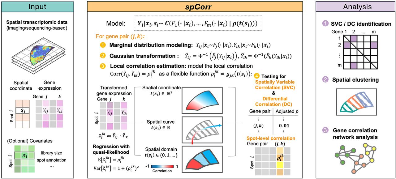
Open in new tab Download PowerPointLink to figure

Estimating the high-dimensional correlation matrix is computationally challenging and often unnecessary, because researchers are typically interested in specific gene pairs (e.g., transcription factor–target, ligand–receptor, etc.). Therefore, spCorr adopts a pairwise strategy instead of estimating the entire high-dimensional correlation matrix. For a gene pair (j, k), the local correlation at spot i is assumed to be

ρ_{i}^{j k} : = {[ρ (t (s_{i}))]}_{j k} = g_{j k} (t (s_{i})),

where g_jk describes how the correlation between genes j and k changes with spatial context.

To accurately estimate the local correlation $ρ_{i}^{j k}$ , spCorr consists of four major steps: marginal distribution modeling, Gaussian transformation, local correlation estimation, and hypothesis testing (Fig. 1, middle). Given a target gene pair (j, k), spCorr performs the following four steps sequentially:

Marginal distribution modeling: For a target gene pair (j, k), the random variables Y_ij and Y_ik, representing the expression of genes j and k at spot i, are modeled separately conditional on spot-level covariates x_i using generalized linear models (GLMs). This yields fitted conditional cumulative distribution functions (CDFs) ${\hat{F}}_{j} (\cdot ∣ x_{i})$ and ${\hat{F}}_{k} (\cdot ∣ x_{i})$ . This step accounts for confounding variation (e.g., library size, spot annotation) that may affect the marginal distribution prior to correlation analysis. It is conceptually similar to the single-cell normalization method sctransform (Hafemeister and Satija 2019), but allows for more flexible specification.
Gaussian transformation: Using the fitted conditional CDFs from Step 1, the counts Y_ij and Y_ik, whose observed values are denoted as y_ij and y_ik, are converted into Gaussian random variables ${\tilde{Y}}_{i j}$ and ${\tilde{Y}}_{i k}$ , whose realizations are denoted as ${\tilde{y}}_{i j}$ and ${\tilde{y}}_{i k}$ . This transformation places both genes on a common Gaussian scale suitable for dependence modeling.
Local correlation estimation: For each spot i, spCorr defines the cross-product of the Gaussian-transformed variables for genes j and k as
$Z_{i}^{j k} = {\tilde{Y}}_{i j} \cdot {\tilde{Y}}_{i k},$
and its realization based on observed data is
$z_{i}^{j k} = {\tilde{y}}_{i j} \cdot {\tilde{y}}_{i k} .$
Under the Gaussian copula framework, the moment properties of $Z_{i}^{j k}$ (in particular its expectation and variance) are directly linked to the local correlation parameter $ρ_{i}^{j k}$ . Therefore, by modeling Z_i as a function of the spatial predictor t(s_i) using a quasi-likelihood generalized additive model, spCorr obtains estimates of the spot-level correlation as an interpretable function of spatial locations
${\hat{ρ}}_{i}^{j k} = {\hat{g}}_{j k} (t (s_{i})),$
where g_jk can be chosen flexibly based on biological contexts.
Hypothesis testing: Finally, spCorr tests if the estimated local correlation varies significantly in space or not. spCorr supports two complementary types of test: (i) testing spatially varying correlation (SVC), which evaluates whether correlations change continuously across spatial coordinates or spatial curves; and (ii) testing differential correlation (DC), which compares correlations between discrete spatial domains.

Downstream analyses supported by spCorr include identifying gene pairs with SVC/DC, spatial clustering based on the spot-level correlation matrix, and gene network analysis (Fig. 1, right). Detailed methodological descriptions are provided in the Methods section. Further evaluation of spCorr through simulation studies and real data applications is presented in the following sections.

Simulations verify spCorr’s reliable FDR control, high power, and computational efficiency

We conducted extensive simulation studies to validate spCorr as an effective method for identifying SVC in ST data, demonstrating reliable FDR control, high statistical power, and computational efficiency. In Simulation Setting 1, to ensure biological realism, we adopted a semi-synthetic simulation framework based on human dorsolateral prefrontal cortex (DLPFC) 10x Genomics Visium data (Maynard et al. 2021), which includes domain annotations (Supplemental Fig. S1). In this context, “semi-synthetic simulation” refers to a framework in which marginal gene expression characteristics (e.g., library sizes, means, and variances) are estimated from real ST data, whereas the gene–gene correlation structure across the space is specified and thus synthetic. From the top 400 spatially variable genes, we selected 200 gene pairs and generated synthetic gene expression using a bivariate Poisson–lognormal model, explicitly dividing them into SVC (spatially varying correlation) and non-SVC (constant correlation) groups. The simulation workflow (Supplemental Fig. S2) combined spot-level library sizes, region-specific gene means (Supplemental Fig. S3), and Poisson sampling to mimic real ST data, and was repeated 30 times to ensure robustness of the evaluation.

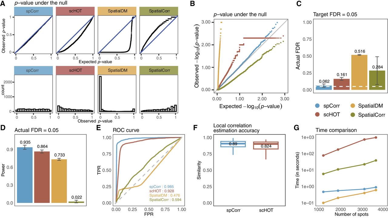
We applied spCorr and three other methods developed for SVC identification and gene local correlation estimation in ST data—scHOT, SpatialDM, and SpatialCorr (Ghazanfar et al. 2020; Bernstein et al. 2022; Li et al. 2023)—to the simulated data. First, we evaluated the validity of these methods’ p-values, which, under the null hypothesis (i.e., this gene pair is not SVC), are expected to follow a Uniform[0,1] distribution. Our results indicate that, among the four methods, spCorr produces the best-calibrated p-values, closely matching the expected uniform distribution (Fig. 2A,B). Among the remaining methods, scHOT and SpatialCorr exhibit substantial deviation from the expected uniform distribution, whereas SpatialDM is completely off with an incorrect concentration of small p-values. Second, we assessed FDR control and statistical power of spCorr compared to the other methods. At a target 5% FDR threshold, spCorr is the only method that effectively controls the false discovery rate, whereas all three alternative methods fail to maintain FDR within the target threshold (Fig. 2C). When comparing statistical power under the 5% FDR threshold, spCorr achieves the highest power (Fig. 2D). Third, we assessed each method’s ability to distinguish SVCs from non-SVCs using the area under the receiver operating characteristic curve (AUROC) as the evaluation metric (Fig. 2E). Our results show that spCorr achieves the highest AUROC values, followed closely by scHOT, whereas SpatialDM and SpatialCorr (Supplemental Fig. S24) show substantially lower performance. These findings highlight spCorr’s superior power and its ability to effectively control the FDR in identifying SVCs. Beyond detection accuracy, we further evaluated the accuracy of spot-level local correlation estimation by comparing the estimated correlations with the ground-truth correlations using cosine similarity (Fig. 2F). spCorr achieves higher similarity to the true correlation structure than scHOT, indicating more accurate recovery of spatially varying correlation patterns. In addition, we compared spCorr against its “without covariate adjustment” version and scHOT, verifying the efficacy of covariate adjustment (Supplemental Figs. S4, S5). Another key advantage of spCorr is its computational efficiency. We compared runtime across increasing numbers of spatial spots and recorded the average computation time per gene pair (Fig. 2G). Although SpatialDM is the fastest method, spCorr demonstrates substantially better scalability than both SpatialCorr and scHOT.

Figure 2.

spCorr achieves reliable FDR control, high statistical power, estimation accuracy, and computational efficiency in simulation studies. (A) Distributions of observed p-values for non-SVC gene pairs across four methods: spCorr, scHOT, SpatialDM, and SpatialCorr. Top: quantile-quantile plots comparing observed p-value quantiles to the expected Uniform[0,1] distribution. Bottom: histograms of observed p-values. spCorr exhibits the closest adherence to the expected Uniform[0,1] distribution, indicating well-calibrated p-values. (B) Quantile-quantile plots of the same p-values as in A on $- \log_{10}$ scale. (C) Actual FDRs achieved by each method under a target FDR of 0.05 (Benjamini–Hochberg adjusted p ≤ 0.05). spCorr shows the most accurate FDR control, whereas all other methods exceed the target FDR threshold. (D) Statistical power of the four methods under the actual FDR = 0.05 cutoff. spCorr achieves the highest power. (E) ROC curves and corresponding AUROC values for the four methods. spCorr attains the highest AUROC among all methods. (F) The accuracy of the local correlation estimation based on cosine similarity. spCorr achieves a higher score compared to scHOT. (G) Runtime (in seconds per gene pair) versus the number of spots. spCorr demonstrates substantially better computational scalability than scHOT and SpatialCorr.

Open in new tab Download PowerPointLink to figure

As complementary evaluations, we considered three additional simulation settings. In Simulation Setting 2, we generated fully synthetic data from a bivariate negative binomial model with spatially varying copula structure, where all model components were specified by fixed parameters rather than derived from real data. spCorr again maintained valid FDR control and achieved the highest power and AUROC (Supplemental Fig. S6). In addition, we verified the validity of spCorr under varying dispersion levels of negative binomial distributions (Supplemental Fig. S7), under zero-inflated negative binomial (ZINB) distributions (Supplemental Fig. S8), and for differential correlation (DC) identification (Supplemental Figs. S9, S10). In all scenarios, spCorr maintained valid FDR control and high statistical power. In Simulation Setting 3, we extended the semi-synthetic framework to a multislide setting by introducing batch effects as slide-level covariates. Because spCorr accommodates arbitrary spot-level covariates in the marginal modeling step, batch effects can be naturally incorporated. As shown in Supplemental Fig. S11, valid FDR control and the highest AUROC are achieved only when both spatial annotation and batch effects are properly adjusted; omitting either covariate leads to inflated FDR and reduced power. In Simulation Setting 4, we further investigated the applicability of spCorr to multislide data sets with spatial misalignment. After applying a spatial alignment method (e.g., Spateo Qiu et al. 2024) and then running the standard spCorr pipeline, spCorr still maintains valid FDR control as well as high power and AUROC value (Supplemental Fig. S12). Full details of the simulation design in all simulation settings are provided in Supplemental Methods S1.1.

In summary, across diverse simulation settings, spCorr outperforms existing methods in SVC/DC detection accuracy while maintaining accurate correlation estimation and strong computational efficiency.

spCorr deciphers heterogeneous regulatory mechanisms within oral squamous cell carcinoma

In our first real-data application, we applied spCorr to ST data of HPV-negative oral squamous cell carcinoma (OSCC) from the 10x Genomics Visium platform (Arora et al. 2023). We used slice 2 as the example, which contains expression measurements for 15,624 genes across 1749 spots. Pathologists divided the Hematoxylin and Eosin (H&E)-stained histological image into six tissue categories, including one tumor region (Tumor) and four non-tumor regions (Fig. 3A). To adjust for potential expression differences between tumor and non-tumor tissues, we included a binary covariate indicating tumor presence in step 1 of spCorr. This helped deconfound correlation estimates and focus the analysis on intratumoral variation. To reduce the search space and focus on biologically relevant interactions, we selected transcription factor (TF)-target gene pairs from the TRRUST v2 database (Han et al. 2018). We further refined this set by removing those regulatory interactions classified as “Repression” and filtered out genes with expression in fewer than 10% of spots.

Figure 3.

spCorr elucidates intratumoral regulatory heterogeneity. (A) H&E-stained image and pathologist-defined spatial annotations for sample 2 of the HPV-negative OSCC data set. The tumor region is distinguished from the surrounding stromal and mucosal tissue. (B) Scatter plots comparing $- \log_{10}$ adjusted p-values from spCorr with those from non-spatial overall correlation (top) and scHOT (bottom) across all candidate TF–target gene pairs. Colors indicate whether a gene pair is identified as significant (BH-adjusted p < 0.05) by spCorr only, by the alternative method only, by both methods, or by neither. (C) GO enrichment analysis of genes identified by two methods. spCorr-identified genes are enriched for epidermis- and keratinocyte-related processes consistent with OSCC biology, whereas genes identified by scHOT show broader and less specific enrichment patterns. (D) Left: Spatial clustering based on spCorr-inferred local correlation estimates reveals tumor subdomains that aligned with original annotations (right) while offering smoother and more clearly defined boundaries. Middle: Louvain clustering based on expression of the same TF-target gene pairs fails to produce comparably distinct boundaries. (E) Spot-level correlation estimates for two representative TF-target pairs. Top: the JUN and CSTA pair exhibits a negative correlation in the tumor core and a positive correlation in the leading edge and transitory region, suggesting localized inflammatory activity in tumor peripheral areas. Bottom: the ELF3 and SPRR1B pair displays a strong positive correlation in the tumor core, consistent with ELF3’s known role in epithelial differentiation. (F) Functional analysis of the ELF3 regulon. Left: GO enrichment analysis of ELF3 regulon reveals biological processes including keratinization and epidermal development. Right: local correlation estimates for ELF3 and its targets are aligned with the boundary of the tumor core, indicating their domain-specific transcriptional activities.

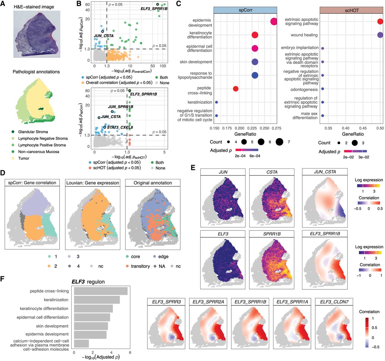
Open in new tab Download PowerPointLink to figure

To assess the utility of spCorr in detecting spatially varying transcriptional regulation, we first compared its output to a standard, non-spatial correlation analysis. When applied to the 1316 candidate TF-target gene pairs, spCorr identified 44 TF-target pairs exhibiting significant SVC at the 5% FDR threshold. For comparison, we also examined gene pairs with significant overall (non-spatial) correlation using a naïve Pearson’s correlation test, as well as gene pairs with significant SVC identified by scHOT. At the 5% FDR threshold, the overall correlation test identifies 417 significant gene pairs (30% of the tested pairs), whereas the scHOT SVC test identifies only 19 significant gene pairs, with the smallest adjusted p-value equal to 0.03, reflecting the limited p-value resolution imposed by the number of permutations in scHOT (Supplemental Fig. S13A; Fig. 3B). In addition, scHOT is substantially more computationally expensive, requiring approximately ten times longer runtime than spCorr (Supplemental Fig. S13B).

Comparing the specific gene pairs identified by the three methods, spCorr uniquely detects several biologically relevant TF-target interactions related to the OSCC tumor context, including JUN_CSTA, JUN_SPRR1B, and STAT3_CXCL8 (Jiang and Li 2022; Karakaslar et al. 2023), which are missed by both the overall correlation analysis and scHOT (Fig. 3B). To further assess the biological relevance of the identified gene pairs, we performed Gene Ontology (GO) functional enrichment analysis on genes identified by spCorr, scHOT, and the overall correlation analysis. Genes identified by spCorr are significantly enriched for biological processes related to epidermis development, keratinocyte differentiation, and epidermal cell differentiation, which are consistent with the epithelial origin of OSCC (Tan et al. 2023). In contrast, genes identified by scHOT and the overall correlation analysis are enriched for more general and heterogeneous biological processes, such as extrinsic apoptotic signaling, wound healing, embryo implantation, and regulation of cell–cell adhesion (Fig. 3C; Supplemental Fig. S13C). Together, these results illustrate the additional biological insight provided by spatially resolved correlation analysis using spCorr.

Next, we explored whether local correlation patterns could reveal spatial heterogeneity within the tumor region. We clustered the spots based on their spCorr-inferred local correlation estimates from the significant SVC pairs using the Louvain algorithm. This correlation-based clustering reveals four distinct spatial domains (Fig. 3D, left) that closely aligned with the annotations reported in the original paper based on multisample integration (Fig. 3D, right). Specifically, clusters 1, 2, and 3 derived from spCorr strongly correspond to the original annotations of the tumor core, transitory region, and leading edge, respectively, while offering smoother patterns and more clearly delineated spatial boundaries. Importantly, this refined clustering is achieved using only a small subset of genes from significant TF-target pairs based on one sample (sample 2), whereas the original annotations rely on whole transcriptomics across twelve samples. In contrast, Louvain clustering based solely on gene expression profiles of the same TF-target pairs results in a less distinct spatial pattern (Fig. 3D, middle). In addition, to provide a comparison with a spatially aware clustering approach, we applied the BANKSY algorithm (Singhal et al. 2024) to the same data set using the same set of TF–target gene pairs. The resulting BANKSY clusters also align with the original annotations; however, the spatial boundaries appear less smooth and less clearly delineated compared to those derived from spCorr-based correlation clustering (Supplemental Fig. S13E, rightmost).

To gain mechanistic insights into local regulatory programs, we investigated local correlation patterns for specific TF-target pairs from spCorr. The pair JUN (also known as c-Jun) and cystatin A (CSTA), for example, exhibited a clear spatial shift in correlation pattern, with a negative correlation in the tumor core that became positive in the leading edge (Fig. 3E, top). This pattern suggests localized activation of inflammatory programs in the peripheral areas of the tumor, as JUN, a key member of the AP-1 complex, has been shown to drive inflammation through increased pro-inflammatory signaling (Karakaslar et al. 2023). Another pair, E74 like ETS transcription factor 3 (ELF3) and small proline rich protein 1B (SPRR1B), showed a strong positive correlation restricted to the tumor core (Fig. 3E, bottom). This may reflect active epithelial differentiation programs, as ELF3 is known to regulate SPRR1B expression in keratinocytes and plays a key role in cornification and epithelial barrier formation (Scholz et al. 2016). To further characterize the regulatory role of ELF3, we extended our analysis from individual gene pairs to its broader set of target genes. Using the spot-level correlation estimates for each TF-target pair, we identified the potential downstream target genes of ELF3, thereby constructing its regulon. GO analysis of the ELF3 regulon showed significant enrichment for biological processes such as keratinization, keratinocyte differentiation, and epidermal cell differentiation (Fig. 3F, left), consistent with previously reported functions of ELF3 (Brembeck et al. 2000). Consistently, the spatial pattern of correlations between ELF3 and its targets aligns closely with the tumor core boundary (Fig. 3F, right), suggesting domain-specific activation of ELF3-regulated transcriptional programs. For comparison, we also visualized the local correlation estimates from scHOT; however, the spatial contrast between the tumor core and leading edge appears less pronounced (Supplemental Fig. S13D), indicating the improved spatial resolution of spCorr in capturing domain-specific regulatory patterns. Lastly, we verified the stability of spCorr: with 200 random runs, the significant SVC pairs are stable (Supplemental Fig. S14; Supplemental Results S2.1).

spCorr uncovers mouse brain cortex functional regions with a limited number of genes

In the second real data application, we applied spCorr to ST data of a coronal section of the mouse brain generated by the 10x Genomics Xenium In Situ technology. Unlike sequencing-based technologies, which measure the whole transcriptome (e.g., 10x Visium in the first real data application), Xenium technology only measures a subset of genes from the pre-defined panel, which is 248 genes in this data set. We focused on studying the cortex structure, thus subsetting a cortex region with 7477 cells. We used two supervised cell type annotation algorithms (Aran et al. 2019; Cable et al. 2022) to obtain faithful cell type labels (Fig. 4A, left). The cell type labels, particularly those corresponding to cortical neurons, clearly align with the six layers of the cerebral cortex (Fig. 4A, right; Allen reference as the ground truth). However, it is easy to notice that the functional region segmentations that are horizontal to the cerebral cortex, for example, Retrosplenial Cortex (RSP), Visual Cortex (VIS), and Primary Somatosensory Cortex (SSp), are not reflected by cell type layers.

Figure 4.

spCorr reveals functional regions within mouse brain cortex layers. (A) Visualization of mouse brain structure. Left: cell type annotation on a Xenium data set. The yellow box shows the cortex region of interest with clear layer structures. Right: reference structure from Allen Brain Atlas. The yellow box is located approximately in the same place as the one on the left. Solid black lines divide adjacent functional regions across layers. (B) Comparison of clustering based on gene expression and spatially varying correlation (SVC). Left: clustering results by Seurat and BANKSY on gene expression and on spCorr-inferred local correlation estimates. Although Seurat and BANKSY clusters on gene expression do not show clear patterns, clusters on SVC exhibit three spatially well-separated clusters. Right: alignment of spCorr-inferred clusters between two adjacent cell type layers. The three clusters in each cell type are well aligned across layers, and roughly match the three functional domains in the Allen Brain Atlas. (C) Visualization of spCorr-inferred local correlation estimates. Top: local correlation estimates of the top ten SVC gene pairs in the original two-dimensional space. Bottom: local correlation estimates of the same gene pairs in the one-dimensional spatial curve space. The shadow labels the 95% confidence interval.

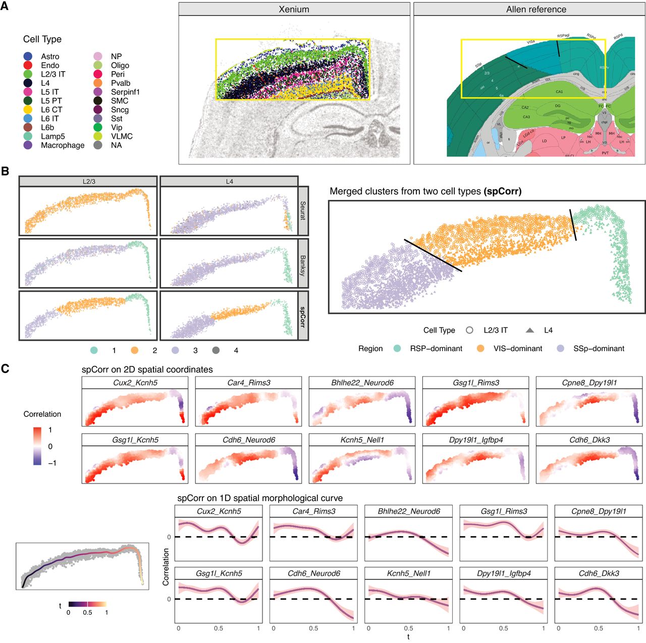
Open in new tab Download PowerPointLink to figure

To explore computational ways to recover these functional regions, we selected the two most abundant layers, L2/3 IT and L4, for further analysis. We first tried Louvain clustering in Seurat based on the 248 genes; Louvain clustering does not show any patterns (Fig. 4B, top left). This result is not surprising, as the panel genes were chosen to distinguish cell types rather than functional regions. We then applied spCorr to each cell type layer separately. No covariates were included or adjusted for in this application, as the analysis was performed separately within each annotated cell type layer to characterize spatial variation in gene–gene correlation within relatively homogeneous cell populations. After gene filtering based on zero proportions to reduce candidate gene pairs, spCorr identified 53 SVC pairs from 8911 gene pairs from L2/3 and 1157 SVC pairs from L4 at the 5% FDR threshold, respectively. Louvain clustering based on spCorr-inferred local correlation estimates from these significant SVC pairs reveals well-separated clusters horizontal to the cortex structure (Fig. 4B, bottom left). Despite clustering being performed independently within each cell type layer, the resulting clusters are highly spatially consistent across the two layers and align closely with the three functional regions—RSP, VIS, and SSp (Fig. 4B, right). In contrast, clustering based on gene expression using the Seurat default Louvain algorithm or the BANKSY method does not align as clearly with these functional regions (Fig. 4B, top left).

To further visualize the SVC patterns, we plotted the local correlation estimates from the top 10 SVC gene pairs in layer L2/3 IT, which have the smallest p-values and largest wiggliness (Fig. 4C, top). Notably, the local correlation estimates for most gene pairs show clear differences between the RSP and VIS regions, even when the marginal expression of the individual genes does not display such a pattern (Supplemental Fig. S15). Considering that the cell type layer has an elongated shape, we applied ideas of the spatial morphological curve from the R package MorphoGAM (Nicol et al. 2024), which reduces the spatial coordinate system from 2 dimensions to 1 dimension (Nicol et al. 2024). spCorr captures similar patterns on this 1D curve as those from 2D space (Fig. 4C, bottom). The 95% confidence intervals provide the local confidence levels of the estimated correlation at each morphological location. Although reflecting similar SVC patterns in 2D space, this 1D “reduced” approach is 15× faster than the 2D case for L2/3 IT and 2× faster for L4. In summary, spCorr expands the feature space by considering gene interactions when the total gene number is limited. The significant SVC patterns on gene pairs reveal important functional regions that are orthogonal to cell types obtained from regular gene-level analysis. Lastly, we extended the clustering analysis to layers L5 and L6. In contrast to L2/3 IT and L4, L5 and L6 contain multiple cell types, which can confound the identification of functional regions. We therefore included cell type labels as covariates in the marginal distribution modeling step of spCorr, and then estimated local correlations and performed Louvain clustering within each layer. In both L5 and L6, the resulting domains showed better separation of functional regions compared with other clustering methods (Supplemental Fig. S16A) and horizontal concordance with the domains identified in L2/3 IT and L4 (Supplemental Fig. S16B).

spCorr discovers biologically relevant correlation shift between mouse hippocampus spatial domains

In the third real-data application, we analyzed a mouse brain hippocampus data set generated with high-resolution 10x Visium HD technology. The original data set includes expression measurements for 18,991 genes across 393,543 spots, captured at an aggregated 8 μm bin resolution. Based on the spatial clustering result (Supplemental Fig. S17), we selected spatially distinct tissue structures that correspond to the pyramidal layer of the hippocampus (Fig. 5A, top), yielding a subset of 5910 spots, as visualized in the corresponding H&E-stained image (Fig. 5A, middle). We further annotated this hippocampal region into CA1, CA2, and CA3 domains based on the expression of canonical marker genes (Supplemental Fig. S18), aligning with the CA1sp, CA2sp, and CA3sp regions defined in the Allen Mouse Brain reference atlas (Wang et al. 2020). Given the slender, curved spatial organization of the CA1–CA3 pyramidal layer, we again applied MorphoGAM (Nicol et al. 2024) to fit a 1D spatial curve that effectively captured the spatial variation along this axis (Fig. 5A, bottom). For gene-level quality control, we retained 964 genes that were expressed in at least 10% of the spots within each of the CA1, CA2, and CA3 domains.

Figure 5.

spCorr discovers biologically relevant correlation shift between spatial domains. (A) Data preprocessing of the Visium HD mouse brain ST data set. Top: spatial segmentation from BANKSY identifying two adjacent domains corresponding to the pyramidal layer of the hippocampus (aligned with CA1sp-CA3sp regions in the Allen Mouse Brain Atlas). Middle: H&E-stained image of the selected hippocampal region. Bottom: spatial annotation based on CA2 marker gene expression and one-dimensional spatial curve fitted by MorphoGAM along the CA1-CA3 axis. (B) Local correlation estimation for representative gene pairs. Top: Log-transformed expression levels of Camk2a, Slc1a2, Ptk2b, and Nrgn. Middle: Scatter plot of the transformed gene expressions after marginal distribution modeling and Gaussian transformation. The black dashed lines indicate ordinary least squares (OLS) regression fits to the scatter plots and are shown for visualization only; the value of ρ displayed in the plot corresponds to the OLS-estimated correlation. Bottom: spCorr-inferred spot-level correlation estimates for each gene pair, with 95% confidence intervals, modeled using discrete spatial domain annotations and visualized along the spatial curve. (C) Differential correlation (DC) analysis between CA1 and CA2. Top: Heatmaps of estimated correlation matrices for significantly DC gene pairs, showing broad downregulation in CA2. Bottom: Hierarchical clustering of the differential correlation matrix identified four gene modules enriched for distinct neuronal processes. (D) Network and functional interpretation of DC results. Top: DC network visualization for gene pairs with statistically significant correlation shifts between CA1 and CA2. Bottom: GO function plot for three representative modules, highlighting synaptic plasticity, synaptic ion signaling, and neuronal structural regulation, which are biological processes known to differ between CA1 and CA2.

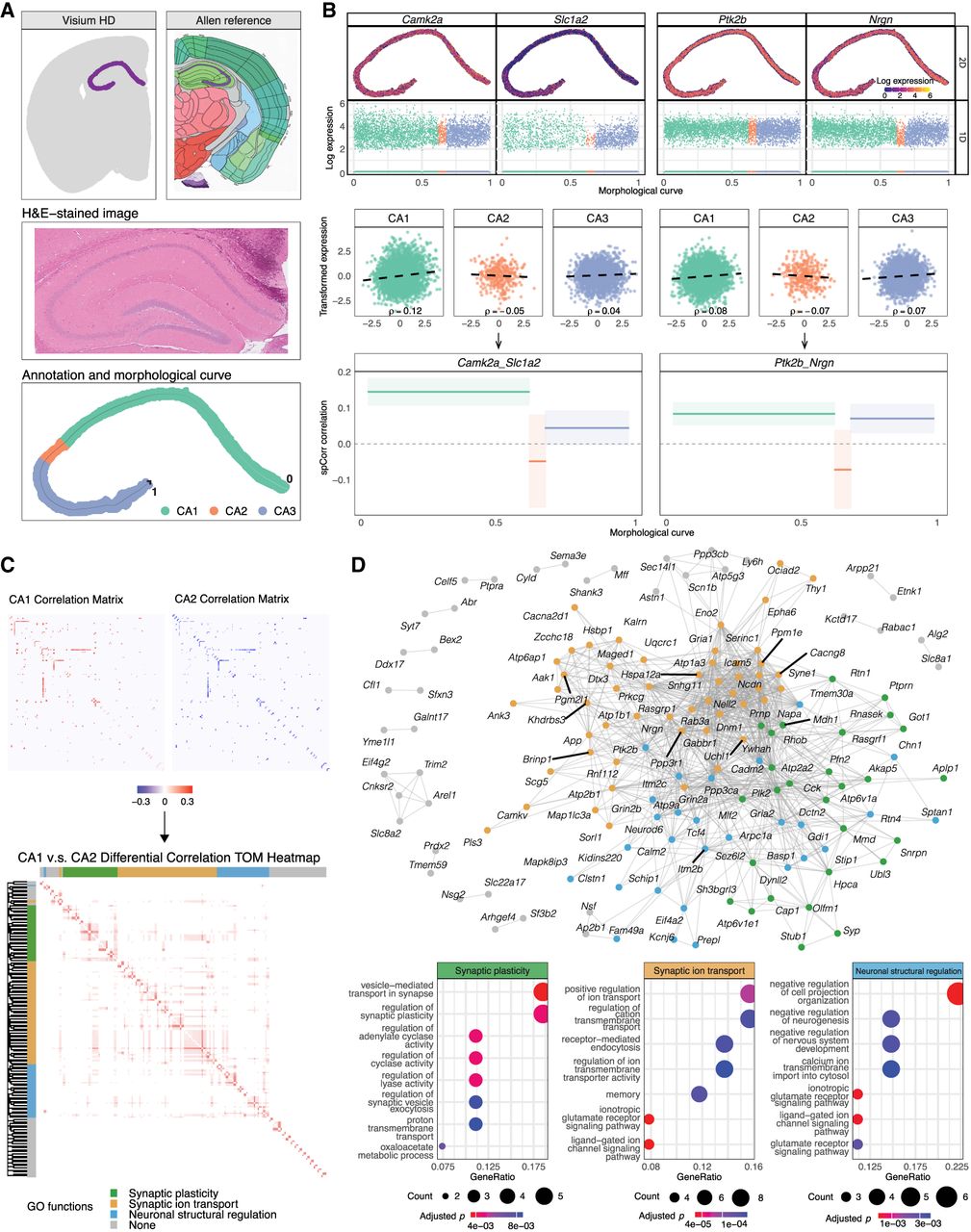
Open in new tab Download PowerPointLink to figure

We next applied spCorr to infer spot-level gene correlations after modeling the marginal distribution given the spatial domain label to adjust average expression differences between the CA1, CA2, and CA3 domains. Specifically, we analyzed 464,166 gene pairs derived from 964 candidate genes. By modeling the correlation as a function of the hippocampal spatial domain annotation and testing whether gene–gene correlations vary across spatial domains, spCorr identifies 5142 gene pairs exhibiting significant SVC at the 5% FDR threshold. For comparison, we also performed SVC testing using the 2D spatial coordinates and the 1D spatial curve representation, testing whether gene–gene correlations vary across continuous 2D space or along the inferred 1D morphological curve. The overlap among gene pairs identified under the three spatial representations is shown in Supplemental Fig. S19, revealing partial overlap as well as unique SVC signals identified by each approach.

To further illustrate how spatial domain annotation informs correlation patterns, we illustrate the spot-level correlation estimation procedure for four representative genes: calcium/calmodulin-dependent protein kinase II alpha (Camk2a), solute carrier family 1 (glial high affinity glutamate transporter), member 2 (Slc1a2), PTK2 protein tyrosine kinase 2 beta (Ptk2b), and neurogranin (Nrgn). The log-transformed gene expression across the 2D spatial coordinates and along the 1D morphological curve is visualized in Fig. 5B (top). After marginal distribution modeling (step 1) and Gaussian transformation (step 2), the transformed gene expressions within each spatial domain (Fig. 5B, middle) are used to infer domain-specific correlation estimates in spCorr. To better visualize the final correlation estimates, we plot spot-level correlation estimates with corresponding 95% confidence intervals for each gene pair along the spatial morphological curve (Fig. 5B, bottom).

To investigate how active gene modules and pathways differ between hippocampal domains, we extended our analysis to differential correlation (DC) testing. A longstanding question in hippocampal neurobiology is whether CA2 represents a functionally distinct region or merely serves as a transition zone between CA1 and CA3. Although CA2 is anatomically positioned between CA1 and CA3 and shares structural features with both, accumulating evidence from pathological and molecular studies supports its classification as a distinct region (Benes et al. 1998; Zhao et al. 2001). Motivated by this, we used spCorr to perform DC testing to determine whether gene correlation patterns differ significantly between CA1 and CA2.

The DC test between CA1 and CA2 identifies 174 significant gene pairs at the 5% FDR threshold, involving 147 unique genes. A heatmap of the estimated correlation matrices for these gene pairs in CA1 and CA2 reveals a clear downregulation in correlation from CA1 to CA2 (Fig. 5C, top). To systematically quantify these differences, we computed a differential correlation matrix by subtracting the estimated correlations in CA2 from those in CA1. We then applied weighted gene correlation network analysis (WGCNA) to the differential correlation matrix, identifying four gene modules via hierarchical clustering of the topological overlap matrix (TOM) (Langfelder and Horvath 2008). To investigate the biological functions associated with these modules, we carried out Gene Ontology (GO) enrichment analysis for each cluster. The results reveal that the modules are significantly enriched for GO terms associated with key neuronal processes, including synaptic plasticity, synaptic ion transport, and neuronal structural regulation (Fig. 5C, bottom). To provide a network-based perspective on these gene correlation changes, we further proposed the gene differential correlation network, where edges represent gene pairs with statistically significant differential correlation, and edge weights reflect the magnitude of correlation difference between CA1 and CA2 (Fig. 5D, top). Previous studies have shown that CA2 neurons exhibit reduced synaptic plasticity and distinct ion signaling dynamics relative to CA1 (Zhao et al. 2007; Simons et al. 2009; Carstens and Dudek 2019). These observations are consistent with our GO enrichment results, as two of the identified modules are significantly associated with synaptic plasticity and ion transport (Fig. 5D, bottom), further supporting previously reported molecular differences between CA1 and CA2.

Additionally, to demonstrate the necessity of the marginal distribution modeling step (step 1) for covariate adjustment in the spCorr pipeline, where marginal distributions were modeled conditional on spatial domain annotations (CA1, CA2, CA3), we conducted a comparative analysis in which this adjustment was omitted. Specifically, we repeated the DC analysis between CA1 and CA2 without accounting for average expression differences between domains in the marginal distribution modeling step. Under this setting, only two gene modules are identified (Supplemental Fig. S20A,B), and functional enrichment is limited, with only one module showing enrichment for known molecular differences between CA1 and CA2 (Supplemental Fig. S20C). In addition, the resulting modules were less clearly separated compared with those obtained using the full spCorr model with covariate adjustment (Fig. 5C,D). These results underscore the importance of properly modeling marginal distributions to uncover biologically meaningful spatially varying correlation patterns.

Although our primary analyses have been focused on the DC analysis between spatial domains in ST data, the spCorr framework is equally applicable to DC analysis between cell types in scRNA-seq data. To demonstrate this generalizability, we applied spCorr to a mouse hippocampus scRNA-seq data set (Saunders et al. 2018). Focusing on annotated pyramidal neurons (CA1, CA2, and CA3 principal cells), we observed similar DC patterns between CA1 and CA2. These DC gene pairs are again enriched for functional categories related to synaptic plasticity and synaptic ion transport (Supplemental Fig. S21), similar to the findings from ST data. This independent analysis reinforces the biological relevance and cross-platform robustness of the DC signals identified by spCorr.

Discussion

We propose a novel statistical framework, spCorr, designed to detect spatially varying correlation (SVC) in spatial transcriptomics data. Unlike existing methods that primarily rely on non-parametric local smoothing, spCorr emphasizes rigorous and interpretable inference through a flexible parametric model. A key innovation of spCorr is its transformation of the pairwise correlation estimation problem into a univariate regression problem. Specifically, spCorr first models each gene’s marginal distribution conditional on potential confounding covariates and transforms gene expression values into standard Gaussian variables. Leveraging Gaussian copula theory, it then constructs a gene-pair cross-product variable and applies a quasi-GAM regression with spatial coordinates as predictors. Finally, spCorr computes p-values in SVC testing using asymptotic theory for quasi-GAMs, and derives the local correlations as an explicit function of spatial location.

Extensive simulations demonstrate that spCorr achieves superior false discovery rate (FDR) control and statistical power compared to state-of-the-art methods like scHOT, SpatialDM, and SpatialCorr. Notably, spCorr is the only method that consistently yields well-calibrated p-values and effectively controls the FDR, even when the data do not perfectly match its model assumptions. This statistical robustness, combined with the flexibility of the GAM framework, enables spCorr to attain the highest power and AUROC across all benchmarks. In real-data applications, spCorr uncovered spatially heterogeneous regulatory patterns and identified spatial domains that were not detectable by conventional gene-level analyses.

A central assumption of spCorr is the Gaussian copula model, which posits that the correlation structure among genes can be represented via a multivariate Gaussian distribution. Our prior work, scDesign3 (Song et al. 2024), established that this model provides a robust and accurate approximation of high-dimensional count data. A unique advantage of the copula framework is its ability to decouple marginal distributions from the dependence structure, allowing spCorr to accommodate a wide range of distributional forms, including Negative Binomial (default for scRNA-seq), Poisson, Zero-Inflated Negative Binomial, Zero-Inflated Poisson, and Gaussian. This decoupling also facilitates the adjustment for arbitrary confounders by modeling each gene’s marginal distribution conditional on covariates—akin to partial correlation in the linear setting.

The decoupling of marginal distributions from the dependence structure has important practical implications. For instance, in our real-data analysis comparing the CA1 and CA2 domains of the mouse hippocampus, we first regressed out the domain labels to equalize each gene’s marginal distribution across domains. This step prevents correlation estimates from being confounded by differences in mean expression levels. Omitting this adjustment would lead the correlation estimates to reflect average expression shifts rather than true domain-specific coordination, resulting in less biologically interpretable gene modules and weaker functional enrichment (Supplemental Fig. S20). This issue, a form of Simpson’s paradox, underscores the critical importance of adjusting for confounding effects. Although spCorr provides flexibility for marginal modeling, we strongly recommend that users carefully choose covariates based on their biological question. In extreme cases, one can even model the marginal distribution as a function of spatial coordinates to remove all spatial effects on gene expression means. A recent preprint adopted this approach to isolate cell-intrinsic coordination by regressing out spatial effects before computing correlation (Vasconcelos et al. 2025).

Beyond marginal modeling, it is also important to distinguish spatially varying correlation (SVC) from differential correlation (DC) across cell types. In gene–gene correlation analyses of ST data, correlation variation may arise from variation in cell type composition across tissue or from continuous spatial effects within cell types, which is analogous to the relationship between spatially variable genes (SVGs) and differentially expressed (DE) genes in gene expression analysis. To disentangle these potential sources of correlation variation, the flexible modeling framework of spCorr enables a principled decomposition of total correlation variation into cell type–associated and continuous spatial components. In Supplemental Results S2.2, we present correlation variation decomposition analyses in the DLPFC 10x Visium (Maynard et al. 2021) and cerebellum Slide-seq (Cable et al. 2022) data sets (Supplemental Figs. S22, S23), showing that although cell type composition often explains a substantial fraction of correlation variation in ST data, continuous spatial effects remain non-negligible beyond cell type effects.

There are several important future directions. Currently, spCorr focuses on gene correlations from spatial transcriptomics. However, to construct more comprehensive gene regulatory networks, integration with additional omics layers—such as chromatin accessibility from spatial ATAC-seq—is necessary. For example, peak-gene correlations have been used to infer cis-regulatory interactions (Granja et al. 2021; Stuart et al. 2021). Extending spCorr to quantify peak-gene correlations in spatial multiomics data (Zhang et al. 2023; Li et al. 2025) is a natural and feasible next step, thanks to the copula model’s flexibility in handling heterogeneous marginal distributions.

Second, the use of regression splines (e.g., thin plate splines and cubic splines) to capture spatial variation assumes smooth spatial surfaces. In reality, tissue structure often leads to abrupt transitions or boundaries in expression patterns. To accommodate such features, future versions of spCorr could incorporate histological images (e.g., H&E staining) to inform spatial discontinuities. In summary, extending spCorr to integrate multimodal spatial data holds great promise for advancing our understanding of spatial gene regulation.

Methods

Mathematical notations

We define a spot as a single observation in a spatial transcriptomics data set. Depending on the technology, a spot may correspond to a capture area (e.g., 10x Visium), a segmented cell (e.g., 10x Xenium), or a bin (e.g., 10x Visium HD). spCorr requires three input matrices: a spot-by-gene expression matrix Y, a spatial coordinate matrix S, and an optional spot-by-covariates matrix X (Fig. 1, left).

First, let $Y = [Y_{i j}] \in R^{n \times m}$ denote the gene expression matrix, where n is the number of spots and m is the number of genes. Likewise, let y = [y_ij] denote the observed gene expression values. Although in this paper we mainly discuss the gene count matrix $Y = [Y_{i j}] \in N^{n \times m}$ , the method is also generalizable to continuous data such as log-transformed gene expression. Second, let $S = {[s_{1}, \dots, s_{n}]}^{⊤} \in R^{n \times 2}$ denote the spatial coordinate matrix, where each $s_{i} = {(s_{i 1}, s_{i 2})}^{⊤}$ specifies the two-dimensional spatial coordinate of spot i. Third, let $X = {[x_{1}, \dots, x_{n}]}^{⊤} \in R^{n \times q}$ denote the matrix of user-defined covariates, where each $x_{i} = {(x_{i 1}, \dots, x_{i q})}^{⊤}$ captures q covariates for spot i that are associated with gene expression (e.g., library size, spot annotation) that may confound the correlation estimation based on the scientific questions.

Gaussian copula model

The spCorr model is formulated using a Gaussian copula (Fig. 1, middle):

Y_{i} ∣ x_{i}, s_{i} \sim C (F_{1} (\cdot ∣ x_{i}), \dots, F_{m} (\cdot ∣ x_{i}) | ρ (t (s_{i}))),

where F_j( · |x_i) is the conditional marginal distribution of gene j given x_i, and C is the Cumulative Distribution Function (CDF) of a multivariate standard Gaussian with correlation matrix ρ(t(s_i)).

The key feature of spCorr is that the correlation matrix is not fixed but varies with spatial predictors t(s_i), which may represent two-dimensional spatial coordinates, one-dimensional spatial curves, or discrete spatial domains. For a gene pair (j, k), the local correlation at spot i is modeled as

ρ_{i}^{j k} : = {[ρ (t (s_{i}))]}_{j k} = g_{j k} (t (s_{i})),

where g_jk describes how local copula correlation between gene j and gene k varies as a function of spatial structure. This pairwise approach enables interpretable and efficient inference of spatial gene–gene relationships.

The spCorr algorithm

The Gaussian copula model defines the overall framework of spCorr. In the following, we describe the implementation of the spCorr algorithm (Fig. 1, middle).

Marginal distribution modeling

For each gene j = 1, …, m at every spot i = 1, …, n, spCorr uses a Generalized Linear Model (GLM) to model the distribution of the observed expression value Y_ij conditional on spot-level covariate x_i:

(1)

{\begin{matrix} Y_{i j} ∣ x_{i} \overset{ind}{\sim} F_{j} (\cdot ∣ x_{i}; μ_{i j}, σ_{i j}) \\ \log (μ_{i j}) = α_{j 0} + f_{j} (x_{i}) \end{matrix}

where F_j( · ; μ_ij, σ_ij) denotes the cumulative distribution function (CDF) of the assumed conditional distribution of Y_ij with mean parameter μ_ij and scale parameter σ_ij. The function f_j(x_i) captures the marginal effect of the spot-level covariates x_i. The specific form of F_j and f_j( · ) depends on the data distribution and the format of covariates, respectively. For instance, if Y is a count matrix, and x_i encodes categorical spatial domain annotations, then F_j is the CDF of a Negative Binomial (NB) distribution, and

f_{j} (x_{i}) = \sum_{k = 1}^{q} x_{i k} β_{k}

is a regression formula on spatial domain annotation. The choice f_j is essentially flexible and may take a nonlinear format, such as a spline, which will change the GLM into a Generalized Additive Model (GAM). spCorr fits the GLM using the R package mgcv, which estimates model parameters by penalized-restricted maximum likelihood estimation (MLE). The fitted CDF for gene j is denoted by

{\hat{F}}_{j} (\cdot ∣ x_{i})

Gaussian transformation

To enable Gaussian copula-based correlation estimation, the observed expression values y_ij are transformed to continuous standard Gaussian variables. Because ST data is often discrete (counts), we first apply a randomized quantile transformation to obtain a continuous uniform variable (Sun et al. 2021; Song et al. 2024):

U_{i j} = (1 - ν_{i j}) F_{j} (Y_{i j} - 1 ∣ x_{i}) + ν_{i j} F_{j} (Y_{i j} ∣ x_{i}), Y_{i j} = 1, 2, \dots

where ν_ij ∼ Uniform[0, 1] is sampled independently. As the true CDF F_j( · |x_i) is unknown, in practice, we use a plug-in estimate based on the fitted CDF

{\hat{F}}_{j} (\cdot ∣ x_{i})

U_{i j} = (1 - ν_{i j}) {\hat{F}}_{j} (Y_{i j} - 1 ∣ x_{i}) + ν_{i j} {\hat{F}}_{j} (Y_{i j} ∣ x_{i}), Y_{i j} = 1, 2, \dots

Each U_ij is then transformed into a standard Gaussian variable using the inverse CDF of the standard Gaussian distribution:

{\tilde{Y}}_{i j} = Φ^{- 1} (U_{i j}),

where Φ( · ) is the CDF of the standard Gaussian distribution. The resulting

{\tilde{Y}}_{i j}

approximately follows a standard Gaussian distribution. To obtain the realization

{\tilde{y}}_{i j}

based on the observed values y_ij, we apply the above transformation:

u_{i j} = (1 - ν_{i j}) {\hat{F}}_{j} (y_{i j} - 1 ∣ x_{i}) + ν_{i j} {\hat{F}}_{j} (y_{i j} ∣ x_{i}), y_{i j} = 1, 2, \dots

and then obtain the Gaussian-scale realization:

{\tilde{y}}_{i j} = Φ^{- 1} (u_{i j}) .

Local correlation estimation

For any gene pair (j, k) at spot i, we consider the bivariate distribution of the transformed expressions $({\tilde{Y}}_{i j}, {\tilde{Y}}_{i k})$ , where both variables approximately follow standard Gaussian distributions: ${\tilde{Y}}_{i j} \sim N (0, 1)$ and ${\tilde{Y}}_{i k} \sim N (0, 1)$ . Their dependence is characterized by the Pearson’s correlation coefficient:

ρ_{i}^{j k} = Corr ({\tilde{Y}}_{i j}, {\tilde{Y}}_{i k}) .

Based on the theory of the Gaussian copula (Nelsen 2006), this quantity is directly related to Kendall’s τ of the original variables via:

τ_{i}^{j k} = \frac{2}{π} \arcsin (ρ_{i}^{j k}),

implying that modeling

ρ_{i}^{j k}

spatially enables estimation of the local Kendall’s τ across the space. To this end, we define a new random variable

Z_{i}^{j k}

, the cross-product of transformed expressions:

Z_{i}^{j k} = {\tilde{Y}}_{i j} \cdot {\tilde{Y}}_{i k},

which, under bivariate normality, satisfies:

E [Z_{i}^{j k}] = ρ_{i}^{j k}, Var (Z_{i}^{j k}) = 1 + {(ρ_{i}^{j k})}^{2} .

This new random variable,

Z_{i}^{j k}

, allows us to convert the modeling of a bivariate distribution into a univariate distribution. The realization

Z_{i}^{j k}

is calculated from the cross-product of transformed observed expression values:

z_{i}^{j k} = {\tilde{y}}_{i j} \cdot {\tilde{y}}_{i k} .

spCorr models the spatial variation in

ρ_{i}^{j k}

as a function of a spatial predictor t(s_i):

ρ_{i}^{j k} = g_{j k} (t (s_{i})),

where t(s_i) is derived from the spatial location s_i. Depending on the application context, this spatial predictor may take one of the following forms:

a two-dimensional spatial coordinate: $t (s_{i}) = (s_{i 1}, s_{i 2}) \in R^{2}$ ,
a one-dimensional spatial morphological curve: $t (s_{i}) = t_{i} \in R$ ,
or a discrete spatial domain label: t(s_i) ∈ {0, 1, …}.

Although it is possible to use MLE to estimate g_jk, the distribution of Z_ij is very complicated, making the computation challenging. However, the variance of Z_ij has a simple relation to its mean, which reminds us of the quasi-likelihood theory as an alternative inference strategy (McCullagh 1983). To estimate $ρ_{i}^{j k}$ , we model the conditional distribution of $Z_{i}^{j k}$ given t(s_i) using a quasi-likelihood generalized additive model (Quasi-GAM). Based on the known mean and variance structure of $Z_{i}^{j k}$ , the corresponding quasi-likelihood function is:

K (Z_{i}^{j k}; ρ_{i}^{j k}) = \int_{ρ_{i}^{j k}}^{Z_{i}^{j k}} \frac{Z - ρ}{1 + ρ^{2}} d ρ + (function of Z_{i}^{j k}) .

Given that spatial predictors may be uncertain (e.g., spatial domain labels may be misannotated), we incorporate observation-specific weights into the quasi-likelihood to account for this uncertainty. Let η_i ∈ [0, 1] denote the uncertainty of the observed spatial predictor t(s_i). We then define the weighted quasi-likelihood contribution as:

K^{'} (Z_{i}^{j k}; ρ_{i}^{j k}) = w_{i} \int_{ρ_{i}^{j k}}^{Z_{i}^{j k}} \frac{Z - ρ}{1 + ρ^{2}} d ρ + (function of Z_{i}^{j k}),

where w_i = 1 − η_i. For spatial domain labels, the uncertainty η_i represents the probability that the annotated domain label does not equal the true label:

η_{i} = 1 - P (t (s_{i}) = t (s_{i}))

. Although the ground-truth uncertainty is typically unknown in practice, it can sometimes be approximated by computational uncertainty scores (Khatri and Bonn 2022; Ergen et al. 2024), and users may also have prior knowledge of regions with unreliable annotations. When such uncertainty estimates are available, this weighting scheme downweights observations with high label uncertainty and improves the robustness of spCorr to noisy spatial annotations.

We then fit a Quasi-GAM by maximizing the quasi-likelihood for each gene pair (j, k) as:

(2)

{\begin{cases} Z_{i}^{j k} ∣ t (s_{i}) are independent, \\ E [Z_{i}^{j k} ∣ t (s_{i})] = ρ_{i}^{j k}, Var (Z_{i}^{j k} ∣ t (s_{i})) = 1 + {(ρ_{i}^{j k})}^{2}, \\ m (ρ_{i}^{j k}) = η_{i}^{j k} = γ_{0}^{j k} + h_{j k} (t (s_{i})), \end{cases}

where

m (\cdot) = artanh (\cdot)

is the hyperbolic arctangent link function mapping (−1, 1) to R, and

γ_{0}^{j k}

is the intercept specific to the gene pair (j, k).

The spatial smoother h_jk(t(s_i)) is defined flexibly depending on the type of spatial predictor t(s_i), which allows spCorr to adapt to diverse spatial structures:

Spatial coordinates ( $t (s_{i}) \in R^{2}$ ): When spatial location is represented by two-dimensional coordinates, h^jk( · ) is modeled using a thin-plate spline. Specifically, it is expressed as a linear combination of radial basis functions:
$h_{j k} (t (s_{i})) = \sum_{l = 1}^{L} β_{l}^{j k} B_{l} (t (s_{i})),$
where $B_{l} : R^{2} \to R$ are pre-defined radial basis functions, and $β_{l}^{j k}$ denotes the coefficient for the lth basis function corresponding to gene pair (j, k).
Spatial curves ( $t (s_{i}) \in R$ ): When spatial variation is captured by a one-dimensional spatial curve, h^jk( · ) is modeled using a univariate cubic spline:
$h_{j k} (t (s_{i})) = \sum_{l = 1}^{L} β_{l}^{j k} b_{l} (t (s_{i})),$
where $b_{l} : R \to R$ are cubic spline basis functions, and $β_{l}^{j k}$ are the corresponding coefficients for gene pair (j, k). Such one-dimensional spatial curves may be defined manually (based on tissue morphology) or inferred computationally (e.g., MorphoGAM Nicol et al. 2024) and then used as the spatial predictors.
Spatial domains (t(s_i) ∈ {0, 1, …, D − 1}): When space is partitioned into discrete domains, h^jk( · ) is modeled as a domain-specific effect using a one-hot encoding:
$h_{j k} (t (s_{i})) = \sum_{l = 1}^{D} β_{l}^{j k} I {t (s_{i}) = l - 1},$
where $I {\cdot}$ is the indicator function, and $β_{l}^{j k}$ represents the corresponding coefficients in domain l for gene pair (j, k).

Model fitting is performed using the mgcv package in R (https://CRAN.R-project.org/package=mgcv). For continuous spatial predictors (e.g., spatial coordinates or morphological curves), the dimension of the basis, denoted by L, controls the flexibility of the smoother. The exact choice of L is typically not critical as long as it is sufficiently large, because spCorr employs penalized maximum likelihood estimation by default to regularize the smoother. This regularization imposes smoothness over space, allowing the model to naturally borrow information from neighboring spatial locations. Disabling the penalty can simplify inference by making p-value computation more straightforward, as it avoids uncertainty due to smoothing parameter estimation. However, doing so may increase the risk of overfitting. For discrete spatial predictors (e.g., spatial domain labels), no penalization is applied, as the smoother reduces to a set of categorical effects.

The final correlation estimate for gene pair (j, k) at spot i is given by

{\hat{ρ}}_{i}^{j k} = m^{- 1} (γ_{0}^{j k} + h_{j k} (t (s_{i}))) = g_{j k} (t (s_{i})),

providing an interpretable function of spatial location for the local correlation between genes j and k, as the model explicitly links correlation strength to spatial predictors such as spatial coordinates, spatial curves, or domain labels.

Hypothesis testing

spCorr supports two types of statistical testing to assess spatial correlation variation for each gene pair (j, k):

Spatially varying correlation (SVC) testing, which evaluates whether correlation varies over continuous spatial predictors (e.g., spatial coordinates or curves).
Differential correlation (DC) testing, which compares the correlation between discrete spatial predictors (e.g., spatial domain labels).

SVC testing

Let ${\hat{β}}^{j k} \in R^{K}$ denote the estimated coefficients of the smooth function h_jk from the Quasi-GAM model. Under regularity conditions, these coefficients satisfy asymptotic normality

{\hat{β}}^{j k} \overset{d}{\to} N (β^{j k}, Var ({\hat{β}}^{j k})) .

The null and alternative hypotheses in testing the SVC are

H_{0} : β^{j k} = 0 vs. H_{1} : β^{j k} \neq 0 .

A significant result indicates that the local correlation

ρ_{i}^{j k}

exhibits spatial heterogeneity.

DC testing

Let d_i ∈ {0, 1, …} denote the discrete spatial domain label for spot i, and let d¹ and d² be two specific domains under comparison. In the Quasi-GAM framework, DC testing evaluates the difference in estimated domain-specific coefficients:

H_{0} : β_{d^{1}}^{j k} = β_{d^{2}}^{j k} vs. H_{1} : β_{d^{1}}^{j k} \neq β_{d^{2}}^{j k} .

Let

{\hat{β}}_{d^{1}}^{j k}

and

{\hat{β}}_{d^{2}}^{j k}

denote the estimated coefficients for domains d¹ and d², respectively. The Wald test statistic is:

W = \frac{{\hat{β}}_{d^{1}}^{j k} - {\hat{β}}_{d^{2}}^{j k}}{\sqrt{Var ({\hat{β}}_{d^{1}}^{j k}) + Var ({\hat{β}}_{d^{2}}^{j k})}}, W \overset{H_{0}}{\sim} N (0, 1) .

The resulting two-sided p-value determines significance; a small p-value indicates evidence of differential correlation between the two spatial domains.

FDR control

For both SVC and DC testing, spCorr applies the Benjamini–Hochberg (BH) procedure (Benjamini and Hochberg 1995) to control the FDR across all tested gene pairs. By default, the FDR threshold is set to 0.05.

Confidence interval

spCorr provides spot-level correlation estimates $ρ_{i}^{j k}$ with uncertainty quantification, that is, confidence intervals for each $ρ_{i}^{j k}$ . Given the fitted value ${\hat{η}}_{i}^{j k}$ and its estimated standard error $\hat{se} ({\hat{η}}_{i}^{j k})$ from the quasi-GAM model (Eq. 2), we first construct a (1 − α) confidence interval for the linear predictor as

{CI}_{1 - α} (η_{i}^{j k}) = [{\hat{η}}_{i}^{j k} - z_{1 - α / 2} \hat{se} ({\hat{η}}_{i}^{j k}), {\hat{η}}_{i}^{j k} + z_{1 - α / 2} \hat{se} ({\hat{η}}_{i}^{j k})],

where z_1−α/2 is the (1 − α/2) quantile of the standard normal distribution.

Then, applying the inverse link function $g^{- 1} (\cdot) = \tanh (\cdot)$ maps the interval back to the correlation scale, yielding the confidence interval for $ρ_{i}^{j k}$ as

{CI}_{1 - α} (ρ_{i}^{j k}) = [\tanh (η_{1}), \tanh (η_{2})],

where

[η_{1}, η_{2}] = {CI}_{1 - α} (η_{i}^{j k})

Downstream analysis

The output of the spCorr algorithm enables several types of downstream analysis (Fig. 1, right).

SVC/DC identification

spCorr identifies informative gene pairs that show significant correlation changes across continuous space (SVC) or between discrete domains (DC). For these gene pairs, the estimated spot-level correlation can be visualized to inspect how functionally related genes correlate across spatial contexts.

Spatial clustering

The estimated local correlation matrices (spot by gene pair) from spCorr can be used for clustering analyses. For example, Louvain clustering applied to these matrices can reveal spatial heterogeneity that may not be apparent from gene expression alone.

Gene correlation network analysis

spCorr also supports network-level analysis. For a given correlation matrix (e.g., from differential correlation), we apply Weighted Gene Correlation Network Analysis (WGCNA) (Langfelder and Horvath 2008). The correlation matrix is first transformed into an adjacency matrix, followed by the computation of the topological overlap matrix (TOM) and corresponding dissimilarity. Hierarchical clustering is then applied to the dissimilarity matrix, and gene modules are identified by dynamic tree cutting.

Data sets

The human dorsolateral prefrontal cortex (DLPFC) 10x Genomics Visium data set (Maynard et al. 2021) used for simulations is accessible through the R package spatialLIBD (Pardo et al. 2022). The human oral squamous cell carcinoma 10x Visium data set (sample 2 from Arora et al. 2023) can be downloaded from Figshare (https://doi.org/10.6084m9.figshare.20304456.v1). The mouse brain cortex 10x Xenium data set is provided by 10x Genomics as part of the “Fresh Frozen Mouse Brain for Xenium Explorer Demo,” available at https://www.10xgenomics.com/datasets/fresh-frozen-mouse-brain-for-xenium-explorer-demo-1-standard. The mouse hippocampus 10x Visium HD data set is also provided by 10x Genomics as part of the “Visium HD Spatial Gene Expression Library, Mouse Brain (FFPE),” available at https://www.10xgenomics.com/datasets/visium-hd-cytassist-gene-expression-libraries-of-mouse-brain-he. The single-cell RNA-seq hippocampus data set from Saunders et al. (2018) is available as a processed Seurat object at https://www.dropbox.com/scl/fi/trw3ujacyi33tawjgd5cr/mouse_hippocampus_reference.rds?rlkey=3gns05ok7qc9cu48voq0atiyp&e=1&dl=0, with raw count matrices downloadable from the DropViz website (http://dropviz.org/). The TRRUST v2 database (Han et al. 2018) used to select transcription factor-target gene pairs can be accessed at https://www.grnpedia.org/trrust/. A detailed summary of all data sets and preprocessing steps is provided in Supplemental Methods S1.2.

Code availability

The spCorr R package is publicly available at GitHub (https://github.com/chexjiang/spCorr) and as Supplemental Code 1. The source code and data required to reproduce all analyses in this study are provided as Supplemental Code 2. All analyses were conducted using R (R Core Team 2024).

Competing interest statement

The authors declare no competing interests.

Acknowledgments

This work was supported by the following grants: UConn Health faculty start-up fund (to D.S.); National Science Foundation DBI-1846216 and DMS-2113754, National Institutes of Health/National Institute of General Medical Sciences R35GM140888, and Silicon Valley Community Foundation 2022-249355 (Chan-Zuckerberg Initiative Single-Cell Biology Data Insights Grant) (to J.J.L.).

Author contributions: C.F.J. and D.S. conceived the study. C.F.J. and D.S. wrote the manuscript. D.S. and J.J.L. revised the manuscript. C.F.J. developed the spCorr R package. C.F.J. and D.S. performed data analysis with assistance from Y.Y. P.R. and Y.J.L. contributed to discussions on real-data applications.

Footnotes

[1] Supplementary material [Supplemental material is available for this article.]

[2] Article published online before print. Article, supplemental material, and publication date are at https://www.genome.org/cgi/doi/10.1101/gr.281559.125.

[3] Freely available online through the Genome Research Open Access option.

References

↵
10x Genomics. 2019. Inside visium spatial capture technology. https://pages.10xgenomics.com/rs/446-PBO-704/images/10x_BR060_Inside_Visium_Spatial_Technology.pdf [accessed April 4, 2025].
Google Scholar
↵
10x Genomics. 2024. Visium HD spatial gene expression performance (technical note CG000686 Rev A). https://cdn.10xgenomics.com/image/upload/v1722285090/support/documents/CG000686_VisiumHDSpatialGeneExpressionPerformance_TechnicalNote_RevA.pdf [accessed April 9, 2025].
Google Scholar
↵
Aran D, Looney AP, Liu L, Wu E, Fong V, Hsu A, Chak S, Naikawadi RP, Wolters PJ, Abate AR, 2019. Reference-based analysis of lung single-cell sequencing reveals a transitional profibrotic macrophage. Nat Immunol 20: 163–172. 10.1038/s41590-018-0276-y
Google Scholar CrossRef PubMed
↵
Arora R, Cao C, Kumar M, Sinha S, Chanda A, McNeil R, Samuel D, Arora RK, Matthews TW, Chandarana S, 2023. Spatial transcriptomics reveals distinct and conserved tumor core and edge architectures that predict survival and targeted therapy response. Nat Commun 14: 5029. 10.1038/s41467-023-40271-4
Google Scholar CrossRef
↵
Benes FM, Kwok EW, Vincent SL, Todtenkopf MS. 1998. A reduction of nonpyramidal cells in sector CA2 of schizophrenics and manic depressives. Biol Psychiatry 44: 88–97. 10.1016/S0006-3223(98)00138-3
Google Scholar CrossRef PubMed Web of Science
↵
Benjamini Y, Hochberg Y. 1995. Controlling the false discovery rate: a practical and powerful approach to multiple testing. J R Stat Soc B 57: 289–300. 10.1111/j.2517-6161.1995.tb02031.x
Google Scholar CrossRef PubMed
↵
Bernstein MN, Ni Z, Prasad A, Brown J, Mohanty C, Stewart R, Newton MA, Kendziorski C. 2022. Spatialcorr identifies gene sets with spatially varying correlation structure. Cell Rep Methods 2: 100369. 10.1016/j.crmeth.2022.100369
Google Scholar CrossRef PubMed
↵
Brembeck FH, Opitz OG, Libermann TA, Rustgi AK. 2000. Dual function of the epithelial specific ets transcription factor, ELF3, in modulating differentiation. Oncogene 19: 1941–1949. 10.1038/sj.onc.1203441
Google Scholar CrossRef PubMed Web of Science
↵
Buphamalai P, Kokotovic T, Nagy V, Menche J. 2021. Network analysis reveals rare disease signatures across multiple levels of biological organization. Nat Commun 12: 6306. 10.1038/s41467-021-26674-1
Google Scholar CrossRef PubMed
↵
Cable DM, Murray E, Zou LS, Goeva A, Macosko EZ, Chen F, Irizarry RA. 2022. Robust decomposition of cell type mixtures in spatial transcriptomics. Nat Biotechnol 40: 517–526. 10.1038/s41587-021-00830-w
Google Scholar CrossRef PubMed
↵
Carstens KE, Dudek SM. 2019. Regulation of synaptic plasticity in hippocampal area CA2. Curr Opin Neurobiol 54: 194–199. 10.1016/j.conb.2018.07.008
Google Scholar CrossRef PubMed
↵
Chen KH, Boettiger AN, Moffitt JR, Wang S, Zhuang X. 2015. Spatially resolved, highly multiplexed rna profiling in single cells. Science 348: aaa6090. 10.1126/science.aaa6090
Google Scholar CrossRef PubMed
↵
Ergen C, Xing G, Xu C, Kim M, Jayasuriya M, McGeever E, Oliveira Pisco A, Streets A, Yosef N. 2024. Consensus prediction of cell type labels in single-cell data with popv. Nat Genet 56: 2731–2738. 10.1038/s41588-024-01993-3
Google Scholar CrossRef
↵
Ghazanfar S, Lin Y, Su X, Lin DM, Patrick E, Han ZG, Marioni JC, Yang JYH. 2020. Investigating higher-order interactions in single-cell data with schot. Nat Methods 17: 799–806. 10.1038/s41592-020-0885-x
Google Scholar CrossRef PubMed
↵
Granja JM, Corces MR, Pierce SE, Bagdatli ST, Choudhry H, Chang HY, Greenleaf WJ. 2021. Archr is a scalable software package for integrative single-cell chromatin accessibility analysis. Nat Genet 53: 403–411. 10.1038/s41588-021-00790-6
Google Scholar CrossRef PubMed
↵
Hafemeister C, Satija R. 2019. Normalization and variance stabilization of single-cell rna-seq data using regularized negative binomial regression. Genome Biol 20: 296. 10.1186/s13059-019-1874-1
Google Scholar CrossRef PubMed
↵
Han H, Cho JW, Lee S, Yun A, Kim H, Bae D, Yang S, Kim CY, Lee M, Kim E, 2018. Trrust v2: an expanded reference database of human and mouse transcriptional regulatory interactions. Nucleic Acids Res 46: D380–D386. 10.1093/nar/gkx1013
Google Scholar CrossRef PubMed
↵
Janesick A, Shelansky R, Gottscho AD, Wagner F, Williams SR, Rouault M, Beliakoff G, Morrison CA, Oliveira MF, Sicherman JT, 2023. High resolution mapping of the tumor microenvironment using integrated single-cell, spatial and in situ analysis. Nat Commun 14: 8353. 10.1038/s41467-023-43458-x
Google Scholar CrossRef PubMed
↵
Jiang M, Li B. 2022. Stat3 and its targeting inhibitors in oral squamous cell carcinoma. Cells 11: 3131. 10.3390/cells11193131
Google Scholar CrossRef
↵
Karakaslar EO, Katiyar N, Hasham M, Youn A, Sharma S, Chung Ch, Marches R, Korstanje R, Banchereau J, Ucar D. 2023. Transcriptional activation of jun and fos members of the ap-1 complex is a conserved signature of immune aging that contributes to inflammaging. Aging Cell 22: e13792. 10.1111/acel.13792
Google Scholar CrossRef PubMed
↵
Karlebach G, Shamir R. 2008. Modelling and analysis of gene regulatory networks. Nat Rev Mol Cell Biol 9: 770–780. 10.1038/nrm2503
Google Scholar CrossRef PubMed Web of Science
↵
Khatri R, Bonn S. 2022. Uncertainty estimation for single-cell label transfer. In Conformal and probabilistic prediction with applications. PMLR 179: 109–128.
Google Scholar
↵
Koplev S, Seldin M, Sukhavasi K, Ermel R, Pang S, Zeng L, Bankier S, Di Narzo A, Cheng H, Meda V, 2022. A mechanistic framework for cardiometabolic and coronary artery diseases. Nat Cardiovasc Res 1: 85–100. 10.1038/s44161-021-00009-1
Google Scholar CrossRef
↵
Langfelder P, Horvath S. 2008. WGCNA: an R package for weighted correlation network analysis. BMC Bioinform 9: 559. 10.1186/1471-2105-9-559
Google Scholar CrossRef PubMed
↵
Li Z, Wang T, Liu P, Huang Y. 2023. Spatialdm for rapid identification of spatially co-expressed ligand–receptor and revealing cell–cell communication patterns. Nat Commun 14: 3995. 10.1038/s41467-023-39608-w
Google Scholar CrossRef PubMed
↵
Li H, Bao S, Farzad N, Qin X, Fung AA, Zhang D, Bai Z, Tao B, Fan R. 2025. Spatially resolved genome-wide joint profiling of epigenome and transcriptome with spatial-ATAC-RNA-seq and spatial-CUT&Tag-RNA-seq. Nat Protoc 20: 2383–2417. 10.1038/s41596-025-01145-9
Google Scholar CrossRef PubMed
↵
Lu S, Keleş S. 2023. Debiased personalized gene coexpression networks for population-scale scRNA-seq data. Genome Res 33: 932–947. 10.1101/gr.277363.122
Google Scholar CrossRef Abstract/Full Text PubMed
↵
Maniatis S, Äijö T, Vickovic S, Braine C, Kang K, Mollbrink A, Fagegaltier D, Andrusivová Ž, Saarenpää S, Saiz-Castro G, 2019. Spatiotemporal dynamics of molecular pathology in amyotrophic lateral sclerosis. Science 364: 89–93. 10.1126/science.aav9776
Google Scholar CrossRef PubMed
↵
Maynard KR, Collado-Torres L, Weber LM, Uytingco C, Barry BK, Williams SR, Catallini JL, Tran MN, Besich Z, Tippani M, 2021. Transcriptome-scale spatial gene expression in the human dorsolateral prefrontal cortex. Nat Neurosci 24: 425–436. 10.1038/s41593-020-00787-0
Google Scholar CrossRef PubMed
↵
McCullagh P. 1983. Quasi-likelihood functions. Ann Stat 11: 59–67. 10.1214/aos/1176346056
Google Scholar CrossRef Web of Science
↵
Mostafavi S, Gaiteri C, Sullivan SE, White CC, Tasaki S, Xu J, Taga M, Klein HU, Patrick E, Komashko V, 2018. A molecular network of the aging human brain provides insights into the pathology and cognitive decline of alzheimer’s disease. Nat Neurosci 21: 811–819. 10.1038/s41593-018-0154-9
Google Scholar CrossRef PubMed
↵
Nelsen RB. 2006. An introduction to copulas. Springer, New York.
Google Scholar
↵
Nicol PB, Ma R, Xu RJ, Moffitt JR, Irizarry RA. 2024. Identifying spatially variable genes by projecting to morphologically relevant curves. bioRxiv 10.1101/2024.11.21.624653
Google Scholar CrossRef Abstract/Full Text
↵
Pardo B, Spangler A, Weber LM, Page SC, Hicks SC, Jaffe AE, Martinowich K, Maynard KR, Collado-Torres L. 2022. spatialLIBD: an R/Bioconductor package to visualize spatially-resolved transcriptomics data. BMC Genomics 23: 434. 10.1186/s12864-022-08601-w
Google Scholar CrossRef PubMed
↵
Qiu X, Zhu DY, Lu Y, Yao J, Jing Z, Min KH, Cheng M, Pan H, Zuo L, King S, 2024. Spatiotemporal modeling of molecular holograms. Cell 187: 7351–7373.e61. 10.1016/j.cell.2024.10.011
Google Scholar CrossRef
↵
Rao A, Barkley D, França GS, Yanai I. 2021. Exploring tissue architecture using spatial transcriptomics. Nature 596: 211–220. 10.1038/s41586-021-03634-9
Google Scholar CrossRef PubMed
↵
R Core Team. 2024. R: a language and environment for statistical computing. R Foundation for Statistical Computing, Vienna. https://www.R-project.org/.
Google Scholar
↵
Rodriques SG, Stickels RR, Goeva A, Martin CA, Murray E, Vanderburg CR, Welch J, Chen LM, Chen F, Macosko EZ. 2019. Slide-seq: a scalable technology for measuring genome-wide expression at high spatial resolution. Science 363: 1463–1467. 10.1126/science.aaw1219
Google Scholar CrossRef PubMed
↵
Saunders A, Macosko EZ, Wysoker A, Goldman M, Krienen FM, de Rivera H, Bien E, Baum M, Bortolin L, Wang S, 2018. Molecular diversity and specializations among the cells of the adult mouse brain. Cell 174: 1015–1030. 10.1016/j.cell.2018.07.028
Google Scholar CrossRef PubMed
↵
Scholz GM, Sulaiman NS, Al Baiiaty S, Kwa MQ, Reynolds EC. 2016. A novel regulatory relationship between ripk4 and elf3 in keratinocytes. Cell Signal 28: 1916–1922. 10.1016/j.cellsig.2016.09.006
Google Scholar CrossRef PubMed
↵
Simons SB, Escobedo Y, Yasuda R, Dudek SM. 2009. Regional differences in hippocampal calcium handling provide a cellular mechanism for limiting plasticity. Proc Natl Acad Sci 106: 14080–14084. 10.1073/pnas.0904775106
Google Scholar CrossRef PubMed
↵
Singhal V, Chou N, Lee J, Yue Y, Liu J, Chock WK, Lin L, Chang YC, Teo EML, Aow J, 2024. Banksy unifies cell typing and tissue domain segmentation for scalable spatial omics data analysis. Nat Genet 56: 431–441. 10.1038/s41588-024-01664-3
Google Scholar CrossRef
↵
Song D, Wang Q, Yan G, Liu T, Sun T, Li JJ. 2024. scdesign3 generates realistic in silico data for multimodal single-cell and spatial omics. Nat Biotechnol 42: 247–252. 10.1038/s41587-023-01772-1
Google Scholar CrossRef
↵
Stuart T, Srivastava A, Madad S, Lareau CA, Satija R. 2021. Single-cell chromatin state analysis with signac. Nat Methods 18: 1333–1341. 10.1038/s41592-021-01282-5
Google Scholar CrossRef PubMed
↵
Su C, Xu Z, Shan X, Cai B, Zhao H, Zhang J. 2023. Cell-type-specific co-expression inference from single cell rna-sequencing data. Nat Commun 14: 4846. 10.1038/s41467-023-40503-7
Google Scholar CrossRef PubMed
↵
Sun T, Song D, Li WV, Li JJ. 2021. scdesign2: a transparent simulator that generates high-fidelity single-cell gene expression count data with gene correlations captured. Genome Biol 22: 163. 10.1186/s13059-021-02367-2
Google Scholar CrossRef PubMed
↵
Tan Y, Wang Z, Xu M, Li B, Huang Z, Qin S, Nice EC, Tang J, Huang C. 2023. Oral squamous cell carcinomas: state of the field and emerging directions. Int J Oral Sci 15: 44. 10.1038/s41368-023-00249-w
Google Scholar CrossRef PubMed
↵
Van Dam S, Vosa U, van der Graaf A, Franke L, de Magalhaes JP. 2018. Gene co-expression analysis for functional classification and gene–disease predictions. Brief Bioinform 19: 575–592. 10.1093/bib/bbw139
Google Scholar CrossRef PubMed
↵
Vasconcelos AG, Danaher P, McGuire D, Wakefield J, Shojaie A. 2025. Accounting for spatial correlation in graphical analysis of spatial transcriptomics data. bioRxiv 10.1101/2025.07.23.666450
Google Scholar CrossRef Abstract/Full Text
↵
Wang X, Allen WE, Wright MA, Sylwestrak EL, Samusik N, Vesuna S, Evans K, Liu C, Ramakrishnan C, Liu J, 2018. Three-dimensional intact-tissue sequencing of single-cell transcriptional states. Science 361: eaat5691. 10.1126/science.aat5691
Google Scholar CrossRef PubMed
↵
Wang Q, Ding SL, Li Y, Royall J, Feng D, Lesnar P, Graddis N, Naeemi M, Facer B, Ho A, 2020. The allen mouse brain common coordinate framework: a 3D reference atlas. Cell 181: 936–953. 10.1016/j.cell.2020.04.007
Google Scholar CrossRef PubMed
↵
Yan G, Hua SH, Li JJ. 2025. Categorization of 34 computational methods to detect spatially variable genes from spatially resolved transcriptomics data. Nat Commun 16: 1141. 10.1038/s41467-025-56080-w
Google Scholar CrossRef PubMed
↵
Yang Y, Han L, Yuan Y, Li J, Hei N, Liang H. 2014. Gene co-expression network analysis reveals common system-level properties of prognostic genes across cancer types. Nat Commun 5: 3231. 10.1038/ncomms4231
Google Scholar CrossRef PubMed
↵
Zhang B, Horvath S. 2005. A general framework for weighted gene co-expression network analysis. Stat Appl Genet Mol Biol 4: Article17. 10.2202/1544-6115.1128
Google Scholar CrossRef PubMed
↵
Zhang S, Yuan L, Danilova L, Mo G, Zhu Q, Deshpande A, Bell AT, Elisseeff J, Popel AS, Anders RA, 2023. Spatial transcriptomics analysis of neoadjuvant cabozantinib and nivolumab in advanced hepatocellular carcinoma identifies independent mechanisms of resistance and recurrence. Genome Med 15: 72. 10.1186/s13073-023-01218-y
Google Scholar CrossRef PubMed
↵
Zhao X, Lein ES, He A, Smith SC, Aston C, Gage FH. 2001. Transcriptional profiling reveals strict boundaries between hippocampal subregions. J Comp Neurol 441: 187–196. 10.1002/cne.1406
Google Scholar CrossRef PubMed Web of Science
↵
Zhao M, Choi YS, Obrietan K, Dudek SM. 2007. Synaptic plasticity (and the lack thereof) in hippocampal CA2 neurons. J Neurosci 27: 12025–12032. 10.1523/JNEUROSCI.4094-07.2007
Google Scholar CrossRef PubMed Web of Science

Method

Flexible and scalable inference of spatially varying correlation in spatial transcriptomics with spCorr

Current Issue:

Abstract

Results

Overview of spCorr method

Simulations verify spCorr’s reliable FDR control, high power, and computational efficiency

spCorr deciphers heterogeneous regulatory mechanisms within oral squamous cell carcinoma

spCorr uncovers mouse brain cortex functional regions with a limited number of genes

spCorr discovers biologically relevant correlation shift between mouse hippocampus spatial domains

Discussion

Methods

Mathematical notations

Gaussian copula model

The spCorr algorithm

Marginal distribution modeling

Gaussian transformation

Local correlation estimation

Hypothesis testing

SVC testing

DC testing

FDR control

Confidence interval

Downstream analysis

SVC/DC identification

Spatial clustering

Gene correlation network analysis

Data sets

Code availability

Competing interest statement

Acknowledgments

Footnotes

References

Article contents

Announcement(s)

Method

Flexible and scalable inference of spatially varying correlation in spatial transcriptomics with spCorr

Cite this article

Share

Current Issue:

Abstract

Results

Overview of spCorr method

Simulations verify spCorr’s reliable FDR control, high power, and computational efficiency

spCorr deciphers heterogeneous regulatory mechanisms within oral squamous cell carcinoma

spCorr uncovers mouse brain cortex functional regions with a limited number of genes

spCorr discovers biologically relevant correlation shift between mouse hippocampus spatial domains

Discussion

Methods

Mathematical notations

Gaussian copula model

The spCorr algorithm

Marginal distribution modeling

Gaussian transformation

Local correlation estimation

Hypothesis testing

SVC testing

DC testing

FDR control

Confidence interval

Downstream analysis

SVC/DC identification

Spatial clustering

Gene correlation network analysis

Data sets

Code availability

Competing interest statement

Acknowledgments

Footnotes

References

Article contents

Announcement(s)