Optimal marker genes for c-separated cell types with SepSolve

Bartol Borozan; Tomislav Prusina; Luka Borozan; Domagoj Ševerdija; Francisca Rojas Ringeling; Domagoj Matijević; Stefan Canzar

doi:10.1101/gr.280637.125

Abstract

The identification of cell types in single-cell RNA-seq studies relies on the distinct expression signature of marker genes. A small set of target genes is also needed to design probes for targeted spatial transcriptomic experiments and to target proteins in single-cell spatial proteomics or for cell sorting. Although traditional approaches have relied on testing one gene at a time for differential expression between a given cell type and the rest, more recent methods have highlighted the benefits of a joint selection of markers that together distinguish all pairs of cell types simultaneously. However, existing methods either consider all pairs of individual cells, which becomes intractable even for medium-sized data sets, or ignore intra-cell-type expression variation entirely by collapsing all cells of a given type to a single representative. Here, we address these limitations and propose to find a small set of genes such that cell types are c-separated in the selected dimensions, a notion introduced previously in learning a mixture of Gaussians. To this end, we formulate a linear program that naturally takes into account expression variation within cell types without including each pair of individual cells in the model, leading to a highly stable set of marker genes that allow to accurately discriminate between cell types and that can be computed to optimality efficiently.

A common first step in the analysis of single-cell data, such as those generated in atlases of the brain and other human organs and tissues (He et al. 2020; Chen et al. 2022), is the characterization of the different cell types and their states based on the distinct expression of so-called marker genes. Typically, cells are first grouped according to their overall transcriptional similarity by a computational clustering method such as Seurat (Hao et al. 2021) and SCANPY (Wolf et al. 2018). Then genes are statistically tested for differential expression between one cluster and the rest (one-vs-rest) (Wolf et al. 2018; Hao et al. 2021), or between all pairs of clusters (package cran) (Lun et al. 2016). The detected marker genes are then used to label and biologically interpret cell clusters in an experimental context. Other general-purpose statistical or machine learning–based methods include the ANOVA F-test and decision trees (Quinlan 1986). Minimum-redundancy-maximum-relevance (mRMR) (Peng et al. 2005), on the other hand, does not only consider the relevance of a feature for an outcome but also takes into account redundancy among features. Similarly, RELIEF (Kononenko 1994) uses nearest neighbors to indirectly account for feature dependencies. Other ranking-based methods include SMaSH (Nelson et al. 2022) and RankCorr (Vargo and Gilbert 2020), which have recently been benchmarked (Pullin and McCarthy 2024) against several other methods. All of these feature-selection methods belong to the class of filter methods that do not interact with a classifier.

Although a one-vs-rest comparison of gene expression allows to differentiate between major cell types, it might fail to detect genes whose expression differs only between similar subtypes, different tissues, or cell types in different disease states (Dumitrascu et al. 2021; Hasanaj et al. 2022). In addition, such a cluster-by-cluster, gene-by-gene approach will introduce redundancy into the set of selected genes, which makes it unsuitable for applications that rely on a small set of informative genes. For example, prominent fluorescence in situ hybridization (FISH)-based spatial transcriptomic technologies can assay only a limited number of genes that need to be preselected. Similarly, fluorescence-activated cell sorting (FACS) relies on a small number of distinct surface markers to sort cells by their types.

Rather than finding genes whose expression is distinct in a given cluster, recent methods have therefore studied a variant of the marker gene selection problem, which seeks to identify a single set of a small number of genes that jointly distinguish all clusters simultaneously. Existing methods model this task as a combinatorial optimization problem and differ mostly in how they measure how much a given gene contributes to the discrimination between two clusters or cell types. scGeneFit (Dumitrascu et al. 2021) and G-PC (Hasanaj et al. 2022) select marker genes such that distances between all pairs of cell types are above a certain threshold. The former method uses a linear program (LP) to minimize, for a fixed number of genes, the violation of the minimum required separation. The latter phrases the problem of minimizing the number of genes necessary to satisfy all distance requirements as a variant of the set cover problem, which it solves using a greedy approach. Similarly, the method used by Langlieb et al. (2023) uses set cover to minimize the number of genes to combinatorially distinguish a given cell type from all others in a single-nucleus RNA-seq data set of the mouse brain. It solves this set cover problem for each cell type using integer linear programming (ILP) and then uses a second ILP to integrate the resulting gene sets while reducing redundancy. To measure the separation between cell types, scGeneFit and G-PC use squared Euclidean or Manhattan distance, respectively, in the dimensions of the selected marker genes. Both methods compute the distance between single representatives (e.g., centroid) of each cell type. Alternatively, scGeneFit allows one to explicitly model the separation of each pair of individual cells from two different types. The combinatorial method used by Langlieb et al. (2023) does not take into account any form of distance between cell types but considers “distinguishable” as a binary property, in which each gene distinguishes between two cell types or not, depending on the difference in the fraction of cells expressing it.

Although one-vs-rest methods based on a statistical test of differential expression naturally take into account expression variation of a given gene across cells of the same type, combinatorial methods that aim to cover or separate all pairs of cell types with a single set of marker genes ignore within-cell-type variation entirely by collapsing all cells of a given type to a single representative. On the other hand, including all pairs of individual cells in an LP, as scGeneFit does, becomes intractable even for small- and medium-sized data sets. It therefore selects a small set of constraints (5000 by default) among typically many millions of possible cell pairs at random, thus ignoring large parts of the generated data. Here we address these limitations and propose a combinatorial method, SepSolve, that takes into account gene expression variation. Our method's objective is to find a small set of genes such that cell types are c-separated in the selected dimensions. In previous work (Dasgupta 2000), two Gaussians have been defined to be c-separated if their centers are c radii apart. Random projection was then used to reduce dimensionality while approximately retaining the separation of a mixture of Gaussians. Instead, here we formulate an ILP based on a linear approximation, which we heuristically solve to search for such a subspace without making the assumption of normality. We provide experimental evidence that this strategy yields a compact, biologically meaningful set of genes that can accurately discriminate between distinct and closely related cell types.

Results

Overview of SepSolve

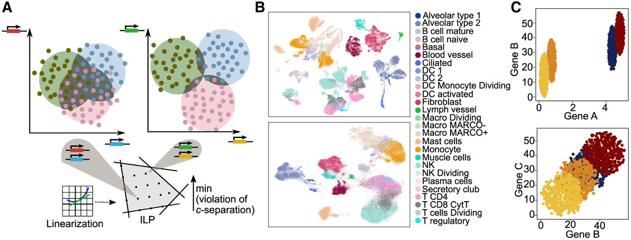
SepSolve is designed to identify a small subset of genes such that the spheres enclosing most of the cells of a given type overlap minimally in the space of selected genes (Fig. 1A). To formalize this objective, we build on the concept of c-separation, as introduced by Dasgupta (2000) for Gaussian mixtures. Specifically, SepSolve achieves c-separation of cell types by selecting genes whose mean expressions are separated by at least the scaled radius of the spheres, with the scaling determined by a separation parameter c. Larger values of c imply stricter separation with less overlap. A two-separated mixture will be almost entirely separated, whereas one- or 1/2-separated clusters will have a small overlap (Dasgupta 2000). The radii of the spheres are calculated using the trace of the covariance matrices, which we demonstrate captures the majority of intra-cell-type expression variation (Methods) (Supplemental Fig. 1).

Figure 1.

SepSolve overview and proof of principle. (A) Overview of the SepSolve algorithm. Using linearizations, SepSolve models the search for marker genes as an integer linear program. Each grid point within the feasible region defined by hyperplanes corresponds to a candidate set of marker genes (two in this example). The optimal solution (here, the highest grid point) minimizes the overlap (dark area) between balls enclosing most cells of a given type, or more formally, minimizes total violation of c-separation between cell types. (B) UMAP embedding of cells in a human lung data set (Madissoon et al. 2020), using 10,000 hvg (top) or 50 markers selected by SepSolve (bottom). (C) Cells from four different types in the projected space of marker genes computed by SepSolve (top) and scGeneFit and G-PC (bottom). The plots show simulated expression levels of two genes (specified on the axes).

Open in new tab Download PowerPointLink to figure

We cast the search for a gene subspace that (almost) induces c-separation as a constrained optimization problem in which, for a given number m of marker genes, the violation of c-separation between pairs of cell types is minimized. After linearizing constraints using Taylor expansions, we obtain an ILP formulation of the problem. Rather than solving it to optimality (e.g., via branch-and-bound), we solve the linear relaxation and select genes corresponding to variables with the m largest values. A detailed description of our method can be found in the Methods.

Figure 1B demonstrates that 50 marker genes selected by SepSolve among 10,000 highly variable genes (hvg) in a human lung scRNA-seq data set (Madissoon et al. 2020) are sufficient to separate cell types in a uniform manifold approximation and projection (UMAP) embedding.

To illustrate the benefits of taking variance into account in the combinatorial model, we have created a synthetic three-dimensional spherical data set consisting of four different labels (i.e., cell types) and three genes, A, B, and C. The mean expression levels of gene A do not differ much between the first two cell types and between the last two, with a difference of only 0.45 units. However, across all cell types, the variance of expression levels of gene A is low, namely, 0.50. The expression means of genes B and C are equidistantly distributed, with a relatively large distance of eight between neighboring cell types. However, the expression of genes B and C exhibit a high variance of 12 across all cell types. As illustrated in Figure 1C, the marker gene selection methods scGeneFit and G-PC, which ignore gene expression variation, choose genes B and C. SepSolve, on the other hand, leverages very small variation in the expression of gene A and selects it as a marker, yielding a much sharper separation of cell types.

SepSolve selects genes that classify cells more accurately

Similar to the benchmarks performed by Dumitrascu et al. (2021) and Hasanaj et al. (2022), we evaluated the discriminatory properties of the identified marker sets by the ability of a classifier to predict cell types based on them.

We compared the performance of SepSolve to most recent combinatorial methods scGeneFit (Dumitrascu et al. 2021) and G-PC (Hasanaj et al. 2022). On smaller data sets, scGeneFit was run in both pairwise and centers mode, including constraints for all pairs of cells or only between single representatives (centers) for each cell type, respectively. The authors’ experiments have shown that the centers mode is the most efficient and stable one. Indeed, attempts to run scGeneFit in pairwise mode on the larger data sets failed because it exceeded available memory or a time limit of 12 h. No implementation of the core combinatorial optimization algorithm described by Langlieb et al. (2023) was available. However, we note that the ILP formulation of Langlieb et al. (2023) tackles a variant of the set cover problem, in the same spirit as G-PC but based on a different notion of distinguishability. In addition, we compared SepSolve with the selection of differentially expressed genes (DEs) and filter methods SMaSH (Nelson et al. 2022), RankCorr (Vargo and Gilbert 2020), mRMR (Peng et al. 2005), and mutual information (Kraskov et al. 2004). SMaSH failed to complete within the 12 h time limit on all but the smallest data set.

We benchmarked methods on seven different scRNA-seq data sets (Table 1). We included all three data sets used by Hasanaj et al. (2022) from the human lung (IPF), mouse cortex (MC), and a human cell atlas (HCA). Consistent with the method of Hasanaj et al. (2022), we restricted the IPF data set to the healthy samples. Although IPF and MC samples were obtained from a single tissue, in HCA identical cell types occurred in multiple tissues. We defined cell-type labels by either merging cell types across tissues or by distinguishing identical cell types originating from different tissues. We used an additional data set (Zheng8eq) of peripheral blood mononuclear cells (PBMCs) in our benchmark, which included both distinct and similar cell types (Pan et al. 2023). We further included two human lung data sets (MaL and MeL) that were used by Kuemmerle et al. (2024) to benchmark the probe set selection method Spapros. We used them in the next section to assess SepSolve's cross-data set classification performance. True cell-type labels were taken from the original publications. In the Zheng8eq data set, the authors randomly mixed roughly equal proportions of presorted B cells, CD14 monocytes, naive cytotoxic T cells, regulatory T cells, CD56 NK cells, memory T cells, CD4 T helper cells, and naive T cells. In this case, true labels were independent of scRNA-seq measurements.

Table 1.

Data sets used in this study

Data set	No. of cells	No. of genes	No. of cell types	References
Idiopathic pulmonary fibrosis (IPF)	96,303	45,947	38	Adams et al. 2020
Human cell atlas (HCA)	84,363	22,653	24/196	He et al. 2020
Mouse cortex (MC)	3005	20,006	7	Zeisel et al. 2015
PBMC (Zheng8eq)	3971	1571	8	Duò et al. 2018
Meyer lung (MeL)	193,108	33,538	80	Madissoon et al. 2023
Madissoon lung (MaL)	57,020	25,204	28	Madissoon et al. 2020
Fetal liver (FL)	113,063	27,080	27	Popescu et al. 2019

[i] For HCA, the number of cell types is shown when merging labels across tissues (24) and when distinguishing the tissue of origin (196).

Open in new tabLink to table

Consistent with the analysis of Dumitrascu et al. (2021) and Hasanaj et al. (2022), we used the marker genes found by each method in k-nearest neighbors (k-NNs) and logistic regression classifiers. For the logistic regression classifier, we split the data into 70% for training and 30% for testing. As in the method of Hasanaj et al. (2022), we measured the performance of the classifiers using the macroaverage F1 score, which corrects for an unbalanced cell-type composition and gives higher weight to rare cell types. It is computed as the mean F1 score across all cell types.

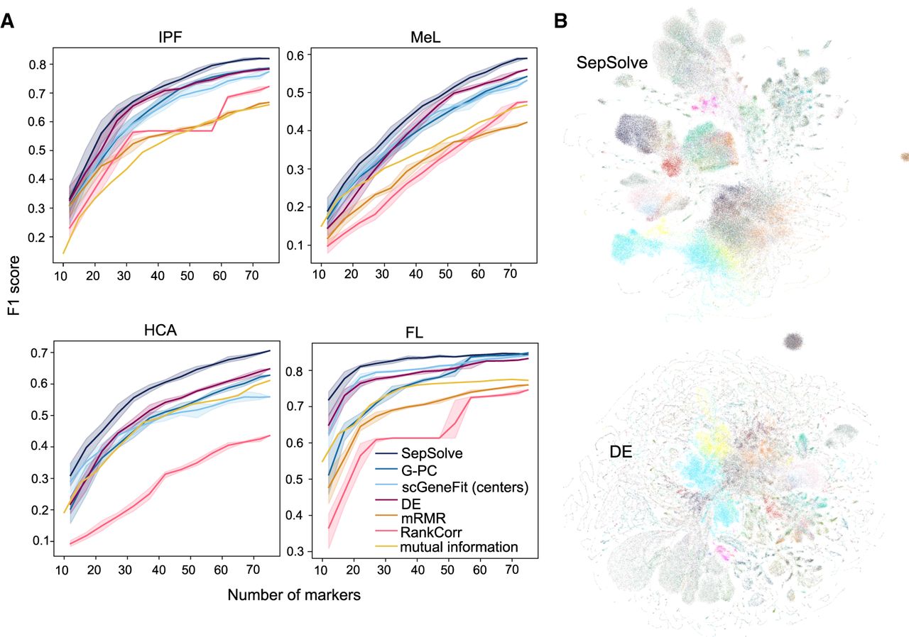
Figure 2A and Supplemental Figure 2 highlight the improved performance of the logistic regression classifier in predicting cell-type labels based on marker genes identified by SepSolve. The increase in F1 score is particularly noticeable when using a small number of marker genes in the FL data set (Fig. 2A) and in the data sets HCA (with merged cell-type labels) and Zheng8eq (Supplemental Fig. 2), in which F1 scores of best-performing methods converge to similar F1 values as the number of markers increases. In contrast, on the HCA (with labels split between tissues), MeL, and IPF data sets (Fig. 2A), SepSolve's improvement over competing methods becomes more pronounced with an increasing number of marker genes. In the case of the MeL data set, cell classification with k-NNs outperforms logistic regression, particularly with a smaller set of markers (Supplemental Fig. 3). For both classifiers, the performance of methods that perform competitively with fewer markers, namely, scGeneGit and mutual information, declines as the number of markers increases. In contrast, DE shows the opposite trend, with performance improving as the number of markers increases but showing worse performance for a small number of markers. Notably, on the Zheng8eq data set (Supplemental Fig. 2), only the performance of DE approaches that of SepSolve, leaving a significant gap between SepSolve and all other methods, including the combinatorial algorithms G-PC and scGeneGit. The smallest improvement can be observed on the IPF data set, but the advantage of our method becomes more evident when using the slightly more accurate k-NN classifier. Overall, using k-NN instead of logistic regression yields consistent results (Supplemental Fig. 3). The MC is the only instance in which SepSolve's gene sets of fewer than 30 genes yielded lower F1 scores than those of the classical differential expression testing (Supplemental Fig. 2). Notably, even RankCorr and mRMR, two of the poorest-performing methods across all other data sets, achieved competitive results on this data set. Notably, SMaSH completed successfully within the 12 h time limit on this data set (it failed on all others) but performed the worst across all tested numbers of marker genes. This finding is consistent with the result of Kuemmerle et al. (2024), in which SMaSH took 15 h to complete on the MeL data set and performed poorly in classification.

Figure 2.

Improvements in cell-type classification and visualization. (A) One scores of a logistic regression classifier when provided varying numbers of marker genes computed by the different methods on the four data sets. On HCA, cell-type labels distinguished the tissue of origin. scGeneFit ran successfully in pairwise mode only on the two smallest data sets, SMaSH only on Zheng8eq (for details, see text). Shaded regions depict standard deviation. (B) UMAP embeddings generated from the 20 marker genes selected by SepSolve and DE on the human lung data set MeL. UMAP embeddings of the original space and of marker genes selected by the remaining methods are in Supplemental Figure 5, along with the complete cell-type legend.

Open in new tab Download PowerPointLink to figure

Even when compared with the recent method Spapros (Kuemmerle et al. 2024), which does not belong to the class of filter methods but uses the results of a classifier to select marker genes, SepSolve's performance is competitive (Supplemental Fig. 4) and again shows advantages for small numbers of marker genes on the three largest data sets (MeL, HCA, and FL). The greatest advantage of SepSolve is evident when distinguishing identical cell types across different tissues in the HCA. On the two smallest data sets, Zheng8eq and MC, classifier-based marker selection by Spapros performed slightly better than SepSolve for certain marker set sizes. However, in principle, access to a classifier could also enhance SepSolve's classification performance by allowing optimization of its separation parameter c (Methods). As shown in Supplemental Figure 4, SepSolve's performance improves slightly on most data sets and substantially on some (HCA, as well as MC for fewer than 30 marker genes) when c is tuned to the classification task. In the same figure, we also compare this strategy to scGeneFit, which supports hyperparameter tuning of its target cell separation parameter via a dual annealing approach. scGeneFit also benefits from classifier-based parameter tuning, especially on data sets Zheng8eq and HCA but does not reach the performance of tuned SepSolve. Among combinatorial methods, scGeneFit is unique in offering built-in hyperparameter optimization.

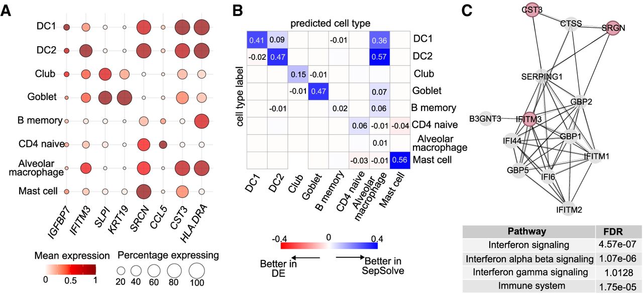
SepSolve's combinatorial gene marker approach enhances the accuracy of cell-type classification in a single-cell lung data set (MeL) even when choosing a limited set of 20 markers (Fig. 2A), underscoring the efficiency of this approach. Overall, this improvement is further supported by a visual comparison of UMAP embeddings generated from the 20 marker genes selected by the top-performing methods (Fig. 2B; Supplemental Fig. 5). For instance, the simultaneous assessment of IFITM3, SRGN, and CST3 expression enables a more accurate distinction between type 1 and type 2 dendritic cells compared with traditional differential expression methods (Fig. 3A,B). Constructing a protein–protein interaction network centered on these three genes reveals an enrichment in interferon signaling pathways (Fig. 3C), which are integral to dendritic cell differentiation (Simmons et al. 2012). This observation underlines the biological relevance of selecting these specific markers.

Figure 3.

Markers selected by SepSolve on the MeL lung single-cell data set. (A) Each dot's color represents the scaled mean expression of a marker within a specific cell type, normalized across all cell types. The size of each dot corresponds to the percentage of cells within that cell type expressing the marker. (B) Confusion matrix heatmap comparing cell classification accuracy between markers identified by SepSolve and those selected via differential expression analysis. Positive values (blue) indicate superior classification accuracy using SepSolve markers, whereas negative values (red) denote better performance with differential expression markers. (C) Protein–protein interaction network centered on IFITM3, SRGN, and CST3, constructed using the STRING database. Nodes represent proteins, and edges denote predicted functional associations based on various evidence types, including curated databases and experimental data. The accompanying table lists pathways enriched within this network, along with their associated false-discovery rate (FDR) values. (DC1) Type 1 dendritic cell, (DC2) type 2 dendritic cell, (DE) differential expression.

Open in new tab Download PowerPointLink to figure

SepSolve performs robustly across data sets, parameters, and perturbations

In the context of feature selection, stability refers to the degree of consistency with which a feature is identified as relevant across different conditions. To be practical, such as when designing probes for a targeted spatial transcriptomic experiment based on a reference scRNA-seq sample, a set of marker genes must not only accurately discriminate between cell types but also remain stable across varying experimental conditions, including the number of profiled cells and different noise levels. Figure 4A shows that markers selected by SepSolve based on one human lung data set can be used to accurately classify cells in another scRNA-seq data set generated from the same tissue. To more comprehensively assess marker stability, we followed the approach of Hasanaj et al. (2022) and calculated the stability of a collection of marker gene sets {S₁, S₂, …, S_n} as the average Jaccard similarity of all pairs of sets:

s = \frac{2}{n (n - 1)} \sum_{i = 1}^{n} \sum_{j > 1}^{n} \frac{| S_{i} \cap S_{j} |}{| S_{i} \cup S_{j} |}

Figure 4.

Stability of selected markers. (A) Cross-data set F1 scores of a logistic regression classifier. SepSolve selected 20 marker genes in the MaL (left) or MeL (right) human lung data set. Classification performance was evaluated either on the same data set (dark blue) or the other (light blue). (B) Stability of 50 marker genes computed by the different methods on random subsamples of cells (top) or perturbed counts (bottom). DE crashed on subsampled IPF data because an insufficient number of cells per cell type remained. (C) F1 scores of a logistic regression and a k-NN classifier on data set IPF when using 50 marker genes selected by SepSolve for varying separation constant c.

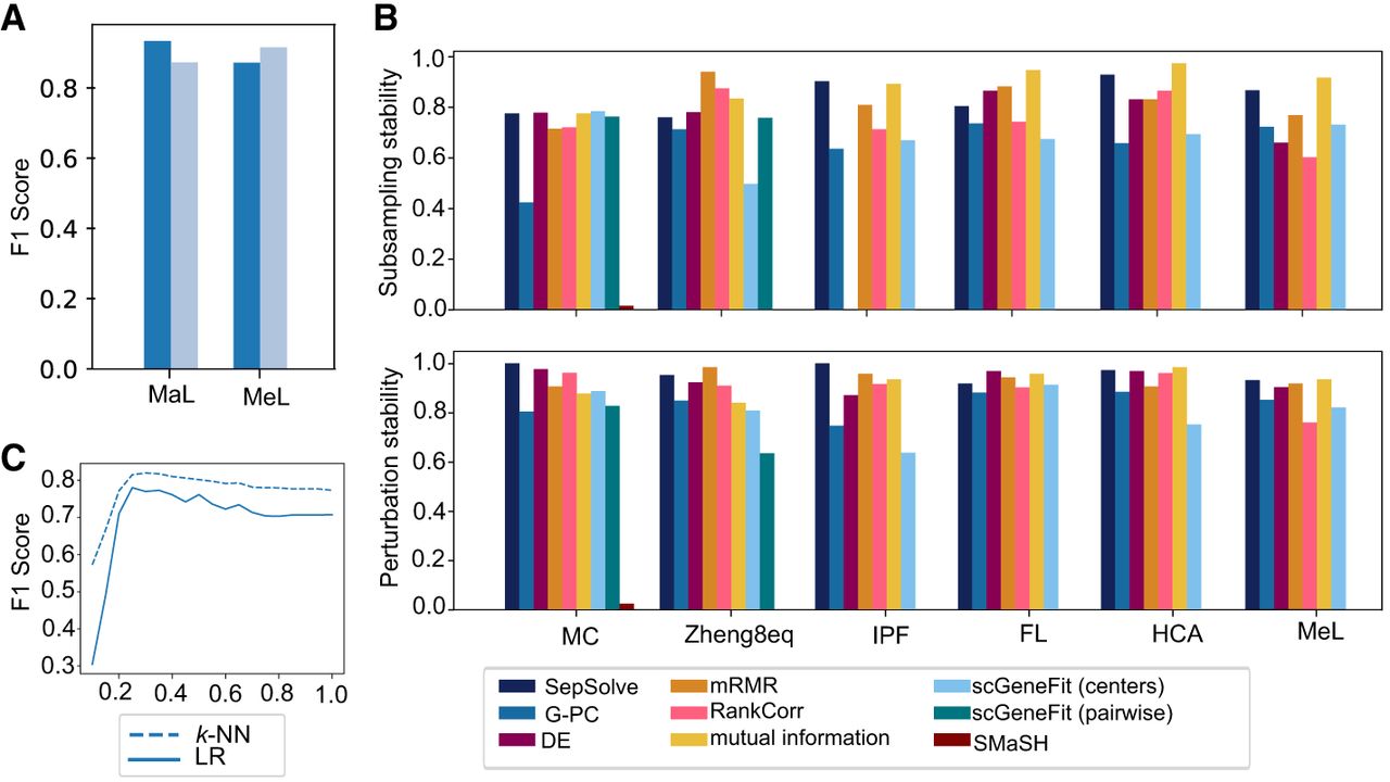
Open in new tab Download PowerPointLink to figure

We evaluated the stability of markers computed by the different methods in two experiments. To avoid a potential confounding influence of the robustness of hvg detection on overall stability, we omitted the selection of hvgs in these experiments. First, consistent with the method of Hasanaj et al. (2022), we randomly sampled 50% of input cells in five random trials. We applied each method to every subsample and then calculated the stability of the marker gene sets identified by each method. Figure 4B (top) shows that SepSolve returns a highly stable set of marker genes with between ∼76% and 93% overlap across all six data sets. The slightly higher stability observed on data sets IPF, HCA, and MeL might be caused by the large number of profiled cells. In contrast, the markers selected by the two combinatorial methods scGeneFit and G-PC showed lower stability across almost all data sets. In the worst case, only half or less than half of marker genes returned by scGeneFit and G-PC overlapped across runs. Notably, taking into account intra-cell-type variability by including constraints between pairs of cells in scGeneFit (pairwise mode) instead of collapsing cell types to a single representative (centers mode) improved scGeneFit's stability (Fig. 4B, top; Supplemental Fig. 6, top). The most stable method is mutual information; however, as shown in the previous section, it did not yield a discriminative set of genes.

In addition, we assessed stability with respect to a small data perturbation. To this end, for each entry e in the raw count matrix, we sampled from a Poisson distribution with expectation 0.05 · e and either added or subtracted the obtained value from the matrix entry with equal probability. Again, this perturbation was applied five times, and the stability of detected markers was evaluated. Overall, the marker gene sets were less impacted by this perturbation compared with the subsampling experiment (Fig. 4B, bottom). Notably, marker genes found by SepSolve exhibited >90% overlap across data sets. Again, combinatorial methods, scGeneFit and G-PC, demonstrated lower stability than SepSolve across all data sets. With 64% and 75%, they achieved the lowest stability values on the IPF data set. Subsampling and permutation stability showed consistent patterns when using 25 instead of 50 markers (Supplemental Fig. 6).

Beyond SepSolve's robustness to data perturbations, we also evaluated its sensitivity to the main algorithmic parameter, the target separation c. As shown in Figure 4C and Supplemental Figure 7, both classifiers maintain consistently high F1 scores when the separation exceeds a minimum threshold of approximately 0.3, with only a gradual decline observed as c increases further.

SepSolve scales to large data sets

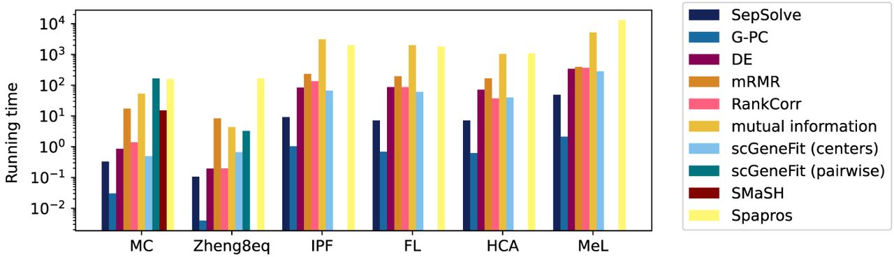
Figure 5 displays the average running times of the different methods across all numbers of target marker genes evaluated in Figure 2 for the six data sets. All experiments were run on an AMD Ryzen Threadripper 3990X 64-core processor @ 4.3 GHz, 256 GB of RAM, and Python version 3.10.12. Except for scGeneFit run in pairwise mode, running times exhibit minimal variability with respect to the number of target genes (Supplemental Fig. 8). As expected, G-PC's greedy heuristic is the fastest, completing in a maximum of 2.46 sec on the largest data set (MeL). SepSolve follows as the second-fastest method. Solving a LP and subsequent rounding in SepSolve took only 49 sec on the largest data set (MeL), whereas scGeneFit, run in the more efficient centers mode, took 285 sec to complete. In pairwise mode, the running time of scGeneFit increased to 160 sec on average on the smaller MC data, with a single instance requiring up to 9206 sec on the same data set. In this mode, scGeneFit failed to run on all but the two smallest data sets owing to memory and time limits (12 h). Similarly, SMaSH successfully ran only on the MC data set. In the work of Kuemmerle et al. (2024), SMaSH took 15 h to find markers in the MeL data set. Spapros, the only non-filter-based method included as a reference in this benchmark, was the slowest method. On the largest lung data set (MeL) it took 13,105 sec (∼3.5 h) to complete compared with under a minute for SepSolve. Even on the smallest MC data set, it required 159 sec, whereas SepSolve completed the task in under a second. With few exceptions, the remaining methods mRMR, RankCorr, DE, and mutual information were at least an order of magnitude slower than SepSolve.

Figure 5.

Average running times (log scale, in seconds) over all evaluated target numbers of marker genes.

Open in new tab Download PowerPointLink to figure

Discussion

We have proposed method SepSolve, a combinatorial approach that tries to discriminate between all cell types simultaneously in the space of marker genes. In contrast to existing methods in this class, it takes into account gene expression variability. Transcriptional heterogeneity within cell types can be owing to different, potentially unknown, cell states and transitions between them but can also have technical reasons such as noisy experimental measurements.

SepSolve annotated cell types more accurately, especially for a small number of marker genes, which is the most common application scenario, for example, when designing probes for a targeted spatial transcriptomic assay. We attribute the higher classification accuracy with fewer markers to SepSolve's combinatorial selection of genes. It allows to discriminate between similar subtypes, which may have overlapping sets of DEs. This was demonstrated by the accurate distinction between closely related type 1 and type 2 dendritic cells in a complex lung data set and by the significant improvement over competing methods when distinguishing identical cell types across different tissues in the HCA. In addition, SepSolve effectively leverages the additional information contained in the within-cell-type expression variation. The value of this is indicated by the substantial improvements in the F1 score by scGeneFit on the Zheng8eq data set, when constraints for all cell pairs (rather than single representatives) were included in an otherwise identical optimization model.

Our method falls under the category of filter methods, which do not optimize a specific classifier during feature selection, in contrast to wrapper and embedded methods (Hasanaj et al. 2022). As a result, the low-dimensional subspace in which we represent cell cluster structures can be beneficial for other tasks, such as the deconvolution of bulk expression data as demonstrated in the work of Hasanaj et al. (2022), or for visualization purposes. Despite this, SepSolve performed favorably in cell-type classification compared with Spapros, a recently proposed embedded method that utilizes the result of a classifier (decision trees) to identify marker genes.

An additional benefit of our method is that it provides a more stable set of markers compared with other combinatorial methods when perturbing or resampling the data. We showed that this also allows for an accurate cross-data set classification of cell types. This is a particularly useful property, for example, when designing spatial probes based on dissociated reference data. Again, we attribute this mainly to taking into account transcriptional heterogeneity within cell types in our model without including every pair of individual cells as scGeneFit does in the pairwise mode. In addition, we optimally solve an LP formulation of the problem compared with the greedy scheme applied by G-PC, which might be more sensitive to small data perturbations (Hasanaj et al. 2022). Nevertheless, like all selection methods, SepSolve will be susceptible to technical variations such as batch effects. Whenever possible, selected genes should be compared across batches.

Furthermore, even though SepSolve takes into account within-cell-type variability, it is fast and can be applied to very large data sets. This is in contrast to scGeneFit, especially when trying to account for expression variability in pairwise mode.

Regarding the selection of the main algorithmic parameter in our method, the target separation c, our experiments showed that a single value, (0.4), effectively produced discriminative sets of marker genes across a diverse range of samples. These included different tissues and species, with varying numbers of profiled cells (ranging from approximately 3000 to 193,000) and cell types (ranging from seven to 38). Furthermore, we showed that beyond a certain minimum threshold, a broad range of values for c yielded similar classification accuracy, highlighting the robustness of the method. However, as shown in Supplemental Figure 4, there exist scenarios in which a tailored choice of c for a specific downstream task (e.g., classification) can significantly enhance SepSolve's performance. Although SepSolve was not originally designed for classifier-specific marker gene selection, the software package provides a grid-search option to fine-tuning c when adapting the method for this purpose.

Furthermore, by leveraging linear programming as the underlying framework for identifying marker genes, SepSolve can seamlessly incorporate prior biological knowledge or technical constraints into the model (Kuemmerle et al. 2024). For instance, disease-relevant genes can be prioritized by setting the corresponding variable to one. This approach ensures that these preselected genes are included, whereas the algorithm identifies additional genes that best complement them, enhancing the relevance and specificity of the selected marker genes.

The number of marker genes required to distinguish cell types depends on several factors, including the intended application and data set characteristics. First, experiments typically impose constraints on the number of marker genes. When designing a targeted spatial experiment, for example, this number is defined by the size of the probe panel. Spapros, for example, was used by Kuemmerle et al. (2024) to find 64 genes that were targeted in a SCRINSHOT (Sountoulidis et al. 2020) experiment on human lung samples.

In addition, the complexity and transcriptional heterogeneity of cell types and the states they are in dictate the necessary number of markers. For example, when aiming to separate only the seven major cell types in our experiments on the MC sample, a straightforward DE approach was sufficient to classify cells with >90% accuracy using just 10 markers. In the original publication (Zeisel et al. 2015), however, 47 subclasses were identified that potentially require not only a larger number but also a combinatorial selection of genes to highlight subtle transcriptional differences between similar subtypes. In such scenarios involving fine-grained cell-type distinctions, our experiments suggest that SepSolve's combinatorial selection of genes reduced the number of genes necessary to distinguish subtle transcriptional differences compared with one-vs-all approaches.

Moreover, the discriminative power of gene sets typically increases with size. But rather than simply increasing the number of genes to achieve a better global separation of cell types, our optimization model can be geared toward the separation of specific cell types that might be known, for example, to be relevant in a given disease context. By introducing a penalty term for the corresponding variable in our objective function, the separation of the two cell types can be forced toward a given target separation. The success of this strategy can be validated by the user by examining the achieved separation for each pair of cell types reported by SepSolve. Future work will focus on tailoring our model to such use cases in complex biological settings.

A current limitation of our method is that total expression variance, namely, the trace of the sample covariance, is used as target separation between cell types, inspired by previous work (Dasgupta 2000) on random projections of high-dimensional Gaussians. Even though we empirically showed that this target separation is justified for single-cell data, more tailored measures might exist. The flexibility of an LP formulation will allow us to investigate alternative measures of separation in future work. A second limitation is the simple ranking scheme we applied to convert fractional solutions of the LP to an integral one. Exact ILP solving with Gurobi already became impractical for moderately sized instances. We will explore more accurate approaches such as branch and bound with heuristic speed-ups and (randomized) rounding schemes with potential guarantees in the future.

Methods

SepSolve optimization

Our approach exploits the notion introduced by Dasgupta (2000) that formalizes that a mixture of Gaussians is c-separated if its component Gaussians are pairwise c-separated.

Definition 1.

Let N(μ₁, Σ₁) and N(μ₂, Σ₂) represent two Gaussians in ℝ^d, where μ₁ and μ₂ are the means and Σ₁, Σ₂ are the covariance matrices, and let () denote the trace of a matrix. We say that two Gaussians are c-separated if

‖ μ_{1} - μ_{2} ‖ \geq c \sqrt{max {tr (Σ_{1}), tr (Σ_{2})}} .

The motivation of Dasgupta (2000) for choosing

\sqrt{tr (Σ)}

as the target separation of the means in the above definition is that tr(Σ) is the expected squared Euclidean distance from the mean:

(1)

E {‖ X - μ ‖}^{2} = tr (Σ) .

Furthermore, for a Gaussian with bounded eccentricity, for which eccentricity was used by Dasgupta (2000) to measure how non-spherical a Gaussian is, the distribution will be concentrated around this radius of

\sqrt{tr (Σ)}

. The degree of separation is controlled by parameter c. Single-cell count data restricted to a single cell type typically do not follow a Gaussian distribution Pan et al. (2023). However, as noted by Dasgupta (2000), random projections of many high-dimensional distributions look more Gaussian owing to the central limit theorem. In fact, in the marker gene subspace we observe (Supplemental Fig. 1) that most of the probability mass lies close to distance

\sqrt{tr (Σ)}

from the mean, rendering Definition 1 suitable as a target separation between cell types.

c-separated point sets in α-subspace

Let S denote a sample of points in ℝ^d. With a slight abuse of notation, below we do not distinguish between population parameters and (estimated) sample statistics. Analogous to Definition 1, we can compute the total sample variance tr(Σ) of S in the following way:

tr (Σ) = \sum_{k = 1}^{d} \sum_{x \in S} \frac{{(x_{k} - μ_{k})}^{2}}{| S | - 1},

where μ denotes the sample mean of set S, k stands for the kth component of a vector in ℝ^d, and |S| denotes the cardinality of S. Let S^α denote the set of points induced by a vector α ∈ {0, 1}^d, such that

S^{α} = {x^{α} \in R^{d} : x_{k}^{α} = α_{k} x_{k}, \forall x \in S} .

Namely, α_k = 1 denotes that the kth coordinate is included, and α_k = 0 denotes that the kth coordinate is ignored. We consider all coordinates for which α_k = 1 to define a point in a α-subspace. Then, the trace of the sample covariance in the α-subspace can be computed as follows:

(2)

t r_{α} (Σ) = \sum_{k = 1}^{d} \sum_{x \in S} \frac{{(α_{k} x_{k} - α_{k} μ_{k})}^{2}}{| S | - 1} = \sum_{k = 1}^{d} α_{k}^{2} \sum_{x \in S} \frac{{(x_{k} - μ_{k})}^{2}}{| S | - 1}

Now, for two samples of points S₁ and S₂, we are ready to rewrite the inequality from Definition 1 in some arbitrary α-subspace:

(3)

\sum_{k = 1}^{d} α_{k}^{2} {(μ_{k}^{(1)} - μ_{k}^{(2)})}^{2} \geq c^{2} max {t r_{α} (Σ_{1}), t r_{α} (Σ_{2})},

where μ⁽¹⁾, μ⁽²⁾ denote the sample means of S₁ and S₂, respectively, and

t r_{α} (Σ_{1})

and

t r_{α} (Σ_{2})

are computed as in Equation 2 for sample covariance matrices Σ₁, Σ₂ of S₁ and S₂, respectively. We call any two point sets S₁ and S₂ in ℝ^d c-separated in α-subspace if Equation 3 holds.

c-separation as optimization problem

To identify an α-subspace of fixed dimension m such that m < d, in which cells of different types achieve c-separation, we formulate a corresponding constrained optimization problem. Specifically, the goal is to minimize a linear objective function that imposes a penalty when the separation of cell types within the α-subspace is not fully realized, subject to a set of nonlinear constraints ensuring distinct separation properties for each cell type. To enable tractable computation, we further linearize these constraints locally around a chosen point, approximating the original problem as an instance of an ILP.

Given input point set S ⊂ ℝ^d, let $S_{i} \subseteq S, i = 1, \dots, l$ , denote all cells of label i. For every pair of sets S_i and S_j, we aim to separate them according to Equation 3. For an arbitrary value of c ∈ ℝ, finding an α-subspace such that all constraints of Equation 3 are satisfied will in general not be feasible. Therefore, we rephrase Equation 3 by introducing slack variables β as follows:

\sum_{k = 1}^{d} α_{k}^{2} {(μ_{k}^{(i)} - μ_{k}^{(j)})}^{2} \geq (c^{2} - β_{i j}) max {t r_{α} (Σ_{i}), t r_{α} (Σ_{j})} .

By increasing values of the slack variables β_ij, we allow for a relaxation of the original requirement that the two sets S_i and S_j must be c-separated. Let L = {{i, j}:i = 1, …, l, j = 1, …, l, i ≠ j} be the set of all unordered pairs of cell labels. We can now formulate the search for an appropriate α-subspace as the following optimization problem:

\begin{matrix} minimize & \sum_{(i, j) \in L} β_{i j} \\ s . t . & \sum_{k = 1}^{d} α_{k}^{2} {(μ_{k}^{(i)} - μ_{k}^{(j)})}^{2} \geq (c^{2} - β_{i j}) max {t r_{α} (Σ_{i}), t r_{α} (Σ_{j})} \forall {i, j} \in L \\ β_{i j} \geq 0 \forall {i, j} \in L \\ α_{k} \in {0, 1} \forall k \in {1, \dots, d} \\ \sum_{k = 1}^{d} α_{k} = m \end{matrix} .

Note that m is the dimension of the subspace induced by the vector α. Furthermore, because α_k can only take the values zero or one, we can substitute

α_{k}^{2}

with α_k in (4). Constraints (4) are not linear because variables β_ij are multiplied with the trace of the covariance matrix of either S_i or S_j, which in turn depend on variables α. Problem (4) is NP-hard (for proof, see Supplemental Material) and cannot be solved efficiently. In fact, the Gurobi QP solver failed to solve even the smallest instances, Zheng8eq and MC, within a full day of computation. To that end, we will linearize the problem in the next section.

LP formulation

In this subsection, we aim to relax our model to enable solving it in polynomial time. Initially, we attempt to convert it into a quadratic program (QP), but we will later show that even the QP is not guaranteed to be polynomial-time solvable. As a result, we further relax the model into a LP, which can be solved efficiently. Let $σ_{k}^{(i)}$ denote the kth diagonal element of the covariance matrix Σ_i, which is given by

σ_{k}^{(i)} = \sum_{x \in S_{i}} \frac{{(x_{k} - μ_{k}^{(i)})}^{2}}{| S_{i} | - 1},

where

μ_{k}^{(i)}

is the mean of gene k across the cells in set S_i, and |S_i| represents the size of S_i. For a fixed α ∈ {0, 1}^d, the trace of the covariance matrix Σ_i is computed as

trac e_{α} Σ_{i} = \sum_{k = 1}^{d} α_{k} σ_{k}^{(i)} .

Relaxation. To simplify the problem, we first relax the binary constraints,

α_{k} \in {0, 1},

to the following box constraints:

α_{k} \in [0, 1] .

This relaxation aims to transform the problem into a QP that can be solved in polynomial time. Next, we attempt to replace the max function present in the constraints.

Max substitution. To replace the constraints involving the max function, we aim to reformulate them in a more computationally tractable form. We begin by observing that the max function can be expressed as

max_{l \in {i, j}} {trac e_{α} (Σ_{l})} = max {\sum_{k = 1}^{d} α_{k} α_{k}^{(i)}, \sum_{k = 1}^{d} α_{k} α_{k}^{(i)}} .

We can distribute the multiplication inside the maximum expression:

(c^{2} - β_{i j}) max {\sum_{k = 1}^{d} α_{k} σ_{k}^{(i)}, \sum_{k = 1}^{d} α_{k} σ_{k}^{(i)}} = max {(c^{2} - β_{i j}) \sum_{k = 1}^{d} α_{k} σ_{k}^{(i)}, (c^{2} - β_{i j}) \sum_{k = 1}^{d} α_{k} σ_{k}^{(i)}} .

To resolve the maximum, we impose that the left-hand side must be greater than or equal to both elements in the maximum expression. This results in the following two constraints:

\begin{aligned} \sum_{k = 1}^{d} α_{k} {(μ_{k}^{(i)} - μ_{k}^{(j)})}^{2} \geq (c^{2} - β_{i j}) \sum_{k = 1}^{d} α_{k} σ_{k}^{(i)}, \\ \sum_{k = 1}^{d} α_{k} {(μ_{k}^{(i)} - μ_{k}^{(j)})}^{2} \geq (c^{2} - β_{i j}) \sum_{k = 1}^{d} α_{k} σ_{k}^{(j)} . \end{aligned}

At this stage, we have a QP. However, these constraints are not convex, meaning the problem is not guaranteed to be polynomial-time solvable. We demonstrate this nonconvexity with a simple example.

Example of nonconvexity. Consider the following example with three genes and two Gaussian distributions:

\begin{aligned} μ_{1} = (\begin{matrix} 0 \\ 0 \\ 0 \end{matrix}), μ_{2} = (\begin{matrix} 1 \\ 1 \\ 1 \end{matrix}), \\ σ_{1} = σ_{2} = (\begin{matrix} 3 & 0 & 0 \\ 0 & 1 & 0 \\ 0 & 0 & 2 \end{matrix}), \end{aligned}

and

c = 1, k = 2.

Substituting these values into the equations results in the following QP:

\begin{aligned} minimize β_{12}, \\ s . t . α_{1} + α_{2} + α_{1} \geq (1 - β_{12}) (3 α_{1} + α_{2} + 2 α_{3}), \\ α_{1} + α_{2} + α_{1} \geq (1 - β_{12}) (3 α_{1} + α_{2} + 2 α_{3}), \\ β_{12} \geq 0, α_{k} \in [0, 1], \\ α_{1} + α_{2} + α_{3} = 2. \end{aligned}

In this case, the points

α_{1} = 1 α_{2} = 0 α_{3} = 1 β_{12} = 0.5

and

α_{1} = 1 α_{2} = 1 α_{3} = 0 β_{12} = 0.5

are feasible. However, their convex combination

α_{1} = 1 α_{2} = 0.5 α_{3} = 0.5 β_{12} = 0.5

is not feasible, as it violates the first constraint

2 \geq 2.5

. This shows that the problem is nonconvex and therefore is not guaranteed to be solvable in polynomial time.

Linearization. To make the problem solvable, we linearize the term involving β_ijα_k using Taylor expansion. Recall the approximation:

β_{i j} α_{k} σ_{k}^{(l)} \approx \frac{1}{2} β_{i j} σ_{k}^{(l)} + \frac{c^{2}}{2} α_{k} σ_{k}^{(l)} - \frac{c^{2}}{4} σ_{k}^{(l)} .

Using this linearization, we can rewrite the original inequality constraints as follows:

\begin{aligned} \sum_{k = 1}^{d} α_{k} {(μ_{k}^{(i)} - μ_{k}^{(j)})}^{2} \geq \sum_{k = 1}^{d} \frac{c^{2}}{2} α_{k} σ_{k}^{(i)} - \frac{1}{2} β_{i j} σ_{k}^{(i)} + \frac{c^{2}}{4} σ_{k}^{(i)}, \\ \sum_{k = 1}^{d} α_{k} {(μ_{k}^{(i)} - μ_{k}^{(j)})}^{2} \geq \sum_{k = 1}^{d} \frac{c^{2}}{2} α_{k} σ_{k}^{(j)} - \frac{1}{2} β_{i j} σ_{k}^{(j)} + \frac{c^{2}}{4} σ_{k}^{(j)} . n \end{aligned} .

LP formulation. Finally, we can formulate the LP as follows. The objective is to minimize the sum of slack variables, β_ij, subject to the following constraints:

\begin{aligned} minimize \sum_{(i, j) \in L} β_{i j}, \\ s . t . \sum_{k = 1}^{d} α_{k} {(μ_{k}^{(i)} - μ_{k}^{(j)})}^{2} \geq \sum_{k = 1}^{d} \frac{c^{2}}{2} α_{k} σ_{k}^{(i)} - \frac{1}{2} β_{i j} σ_{k}^{(l)} + \frac{c^{2}}{4} σ_{k}^{(i)}, \forall (i, j) \in L, \\ \sum_{k = 1}^{d} α_{k} {(μ_{k}^{(i)} - μ_{k}^{(j)})}^{2} \geq \sum_{k = 1}^{d} \frac{c^{2}}{2} α_{k} σ_{k}^{(j)} - \frac{1}{2} β_{i j} σ_{k}^{(l)} + \frac{c^{2}}{4} σ_{k}^{(j)}, \forall (i, j) \in L, \\ β_{i j} \geq 0, \forall (i, j) \in L, \\ α_{k} \in [0, 1], \forall k \in {1, \dots, d}, \\ \sum_{k = 1}^{d} α_{k} = m . \end{aligned}

Benchmarks

Methods

We implemented the ILP described in the previous section in our computational method, SepSolve. We used Gurobi (https://www.gurobi.com) to solve its linear relaxation and convert fractional α to integral values through a simple ranking method that rounds the m largest values to one and sets the remaining α-variables to zero. The same rounding scheme was applied by Dumitrascu et al. (2021). When comparing with embedded method Spapros and with scGeneFit's hyperparameter optimization in Supplemental Figure 4, we tuned the parameter c by interacting with a classifier. Specifically, we split the data into 40% training, 30% validation, and 30% test sets. For each candidate c between 0.1 and one, marker genes were selected, and a logistic regression model was trained on the training set and evaluated by F1 score on the validation set. The best c was then reapplied for marker gene selection and model training on train+validation, and the performance was reported on the held-out test set.

Most methods, including SepSolve, were run using default values for all parameters. In SepSolve we set the default value for the separation constant c to 0.4. The authors of G-PC did not provide a default value for the coverage factor (K) in their implementation. Consistent with the work of Hasanaj et al. (2022), we therefore varied K in the range of {5, …, 20} and chose the value that yielded the highest average accuracy on the IPF data set. The same value was then applied to all data sets.

When running mRMR, we performed a binary search over the parameter lambda to find the value that yields the desired number of marker genes. If no such value exists, we selected the value that produces the largest set of marker genes smaller than the target number of genes. Spapros was run in the cell-type recovery mode (SpaprosCTo). DE genes were obtained using the rank_genes_groups function from the SCANPY package with the default t-test method by sequentially selecting the highest-ranked gene for each cell type until the desired number of marker genes was obtained. Methods were downloaded from the repositories listed in Table 2.

Table 2.

Methods used in this study

Method	Source	GitHub/GitLab
scGeneFit	Dumitrascu et al. 2021	https://github.com/solevillar/scGeneFit-python
G-PC	Hasanaj et al. 2022	https://github.com/euxhenh/phenotype-cover
mRMR	Peng et al. 2005	https://github.com/smazzanti/mrmr
RankCorr	Vargo and Gilbert 2020	https://github.com/ahsv/RankCorr
Spapros	Kuemmerle et al. 2024	https://github.com/theislab/spapros
SMaSH	Nelson et al. 2022	https://gitlab.com/cvejic-group/smash
Mutual Inf.	Pedregosa et al. 2011	https://github.com/scikit-learn/scikit-learn
DE genes	Wolf et al. 2018	https://github.com/scverse/scanpy

Open in new tabLink to table

Data processing

Following the same preprocessing steps as applied by Hasanaj et al. (2022) for assessing classification performance, we removed cell types with fewer than 50 cells and genes expressed in fewer than 10 cells. We omitted the step of cell-type removal when assessing the stability of marker selection. Counts were normalized to 10,000 using the SCANPY Python package and log-transformed after adding a pseudocount of one. Finally, we identified highly variable genes using the highly_variable_genes function from SCANPY, applying the same parameters as those used by Hasanaj et al. (2022) for all data sets. Following the authors’ recommendation, we have additionally standardized the data to zero mean and unit variance when running G-PC. When testing SepSolve's marker genes across the two lung data sets (Fig. 4A), we considered only the cell types and genes common to both data sets.

Software availability

The SepSolve software is available at GitHub (https://github.com/bborozan/SepSolve) and as Supplemental Code.

Competing interest statement

The authors declare no competing interests.

Acknowledgments

We thank the members of the Canzar group for their valuable feedback and the anonymous reviewers for their constructive comments on earlier versions of this manuscript.

Author contributions: All authors conceived the algorithm. B.B. performed the computational experiments. All authors wrote the manuscript. D.M. and S.C. supervised the study.

Notes

[2] Supplementary material [Supplemental material is available for this article.]

[3] Article published online before print. Article, supplemental material, and publication date are at https://www.genome.org/cgi/doi/10.1101/gr.280637.125.

References

↵
Adams TS, Schupp JC, Poli S, Ayaub EA, Neumark N, Ahangari F, Chu SG, Raby BA, DeIuliis G, Januszyk M, 2020. Single-cell RNA-seq reveals ectopic and aberrant lung-resident cell populations in idiopathic pulmonary fibrosis. Sci Adv 6: eaba1983. 10.1126/sciadv.aba1983
Google Scholar CrossRef PubMed
↵
Chen S, Luo Y, Gao H, Li F, Chen Y, Li J, You R, Hao M, Bian H, Xi X, 2022. hECA: the cell-centric assembly of a cell atlas. iScience 25: 104318. 10.1016/j.isci.2022.104318
Google Scholar CrossRef
↵
Dasgupta S. 2000. Experiments with Random Projection. In Proceedings of the 16th Conference on Uncertainty in Artificial Intelligence. UAI ’00, pp. 143–151. Morgan Kaufmann Publishers, San Francisco.
Google Scholar
↵
Dumitrascu B, Villar S, Mixon DG, Engelhardt BE. 2021. Optimal marker gene selection for cell type discrimination in single cell analyses. Nat Commun 12: 1186. 10.1038/s41467-021-21453-4
Google Scholar CrossRef PubMed
↵
Duò A, Robinson MD, Soneson C. 2018. A systematic performance evaluation of clustering methods for single-cell RNA-seq data. F1000Res 7: 1141. 10.12688/f1000research.15666.2
Google Scholar CrossRef PubMed
↵
Hao Y, Hao S, Andersen-Nissen E, Mauck WM, Zheng S, Butler A, Lee MJ, Wilk AJ, Darby C, Zager M, 2021. Integrated analysis of multimodal single-cell data. Cell 184: 3573–3587.e29. 10.1016/j.cell.2021.04.048
Google Scholar CrossRef PubMed
↵
Hasanaj E, Alavi A, Gupta A, Póczos B, Bar-Joseph Z. 2022. Multiset multicover methods for discriminative marker selection. Cell Rep Methods 2: 100332. 10.1016/j.crmeth.2022.100332
Google Scholar CrossRef PubMed
↵
He S, Wang L-H, Liu Y, Li Y-Q, Chen H-T, Xu J-H, Peng W, Lin G-W, Wei P-P, Li B, 2020. Single-cell transcriptome profiling of an adult human cell atlas of 15 major organs. Genome Biol 21: 294. 10.1186/s13059-020-02210-0
Google Scholar CrossRef PubMed
↵
Kononenko I. 1994. Estimating attributes: analysis and extensions of RELIEF. In Machine learning: ECML-94 (ed. Bergadano F, De Raedt L), pp. 171–182. Springer, Berlin.
Google Scholar
↵
Kraskov A, Stögbauer H, Grassberger P. 2004. Estimating mutual information. Phys Rev E 69: 066138. 10.1103/PhysRevE.69.066138
Google Scholar CrossRef PubMed
↵
Kuemmerle LB, Luecken MD, Firsova AB, Barros de Andrade e Sousa L, Straßer L, Mekki II, Campi F, Heumos L, Shulman M, Beliaeva V, 2024. Probe set selection for targeted spatial transcriptomics. Nat Methods 21: 2260–2270. 10.1038/s41592-024-02496-z
Google Scholar CrossRef
↵
Langlieb J, Sachdev NS, Balderrama KS, Nadaf NM, Raj M, Murray E, Webber JT, Vanderburg C, Gazestani V, Tward D, 2023. The molecular cytoarchitecture of the adult mouse brain. Nature 624: 333–342. 10.1038/s41586-023-06818-7
Google Scholar CrossRef PubMed
↵
Lun A, McCarthy D, Marioni J. 2016. A step-by-step workflow for low-level analysis of single-cell RNA-seq data with Bioconductor. F1000Res 5: 2122. 10.12688/f1000research.9501.2
Google Scholar CrossRef PubMed
↵
Madissoon E, Wilbrey-Clark A, Miragaia RJ, Saeb-Parsy K, Mahbubani KT, Georgakopoulos N, Harding P, Polanski K, Huang N, Nowicki-Osuch K, 2020. scRNA-seq assessment of the human lung, spleen, and esophagus tissue stability after cold preservation. Genome Biol 21: 1. 10.1186/s13059-019-1906-x
Google Scholar CrossRef PubMed
↵
Madissoon E, Oliver AJ, Kleshchevnikov V, Wilbrey-Clark A, Polanski K, Richoz N, Ribeiro Orsi A, Mamanova L, Bolt L, Elmentaite R, 2023. A spatially resolved atlas of the human lung characterizes a gland-associated immune niche. Nat Genet 55: 66–77. 10.1038/s41588-022-01243-4
Google Scholar CrossRef PubMed
↵
Nelson ME, Riva SG, Cvejic A. 2022. SMaSH: a scalable, general marker gene identification framework for single-cell RNA-sequencing. BMC Bioinformatics 23: 328. 10.1186/s12859-022-04860-2
Google Scholar CrossRef PubMed
↵
Pan Y, Justin TL, Moorad R, Wu D, Marron JS, Dittmer DP. 2023. The Poisson distribution model fits UMI-based single-cell RNA-sequencing data. BMC Bioinformatics 24: 256. 10.1186/s12859-023-05349-2
Google Scholar CrossRef PubMed
↵
Pedregosa F, Varoquaux G, Gramfort A, Michel V, Thirion B, Grisel O, Blondel M, Prettenhofer P, Weiss R, Dubourg V, 2011. Scikit-learn: machine learning in Python. J Mach Learn Res 12: 2825–2830.
Google Scholar CrossRef PubMed
↵
Peng H, Long F, Ding C. 2005. Feature selection based on mutual information criteria of max-dependency, max-relevance, and min-redundancy. IEEE Trans Pattern Anal Mach Intell 27: 1226–1238. 10.1109/TPAMI.2005.159
Google Scholar CrossRef PubMed Web of Science
↵
Popescu DM, Botting RA, Stephenson E, Green K, Webb S, Jardine L, Calderbank EF, Polanski K, Goh I, Efremova M, 2019. Decoding human fetal liver haematopoiesis. Nature 574: 365–371. 10.1038/s41586-019-1652-y
Google Scholar CrossRef PubMed
↵
Pullin JM, McCarthy DJ. 2024. A comparison of marker gene selection methods for single-cell RNA sequencing data. Genome Biol 25: 56. 10.1186/s13059-024-03183-0
Google Scholar CrossRef PubMed
↵
Quinlan JR. 1986. Induction of decision trees. Mach Learn 1: 81–106. 10.1023/A:1022643204877
Google Scholar CrossRef
↵
Simmons DP, Wearsch PA, Canaday DH, Meyerson HJ, Liu YC, Wang Y, Boom WH, Harding CV. 2012. Type I IFN drives a distinctive dendritic cell maturation phenotype that allows continued class II MHC synthesis and antigen processing. J Immunol 188: 3116–3126. 10.4049/jimmunol.1101313
Google Scholar CrossRef PubMed
↵
Sountoulidis A, Liontos A, Nguyen HP, Firsova AB, Fysikopoulos A, Qian X, Seeger W, Sundström E, Nilsson M, Samakovlis C. 2020. SCRINSHOT enables spatial mapping of cell states in tissue sections with single-cell resolution. PLoS Biol 18: e3000675. 10.1371/journal.pbio.3000675
Google Scholar CrossRef PubMed
↵
Vargo AHS, Gilbert AC. 2020. A rank-based marker selection method for high throughput scRNA-seq data. BMC Bioinformatics 21: 477. 10.1186/s12859-020-03641-z
Google Scholar CrossRef PubMed
↵
Wolf FA, Angerer P, Theis FJ. 2018. SCANPY: large-scale single-cell gene expression data analysis. Genome Biol 19: 15. 10.1186/s13059-017-1382-0
Google Scholar CrossRef PubMed
↵
Zeisel A, Muñoz-Manchado AB, Codeluppi S, Lönnerberg P, La Manno G, Juréus A, Marques S, Munguba H, He L, Betsholtz C, 2015. Cell types in the mouse cortex and hippocampus revealed by single-cell RNA-seq. Science 347: 1138–1142. 10.1126/science.aaa1934
Google Scholar CrossRef PubMed

Method

Optimal marker genes for c-separated cell types with SepSolve

Current Issue:

Abstract

Results

Overview of SepSolve

SepSolve selects genes that classify cells more accurately

SepSolve performs robustly across data sets, parameters, and perturbations

SepSolve scales to large data sets

Discussion

Methods

SepSolve optimization

c-separated point sets in α-subspace

c-separation as optimization problem

LP formulation

Benchmarks

Methods

Data processing

Software availability

Competing interest statement

Acknowledgments

Notes

References

Article contents

Announcement(s)

Method

Optimal marker genes for c-separated cell types with SepSolve

Cite this article

Share

Current Issue:

Abstract

Results

Overview of SepSolve

SepSolve selects genes that classify cells more accurately

SepSolve performs robustly across data sets, parameters, and perturbations

SepSolve scales to large data sets

Discussion

Methods

SepSolve optimization

c-separated point sets in α-subspace

c-separation as optimization problem

LP formulation

Benchmarks

Methods

Data processing

Software availability

Competing interest statement

Acknowledgments

Notes

References

Article contents

Announcement(s)