
Comprehensive identification of genomic and environmental determinants of phenotypic plasticity in maize
- 1Department of Agronomy, Iowa State University, Ames, Iowa 50011, USA;
- 2USDA-ARS, Wheat Health, Genetics, and Quality Research Unit, Pullman, Washington 99164, USA;
- 3USDA-ARS, Corn Insects and Crop Genetics Research Unit, Ames, Iowa 50011, USA;
- 4National Key Laboratory of Crop Genetic Improvement, Huazhong Agricultural University, Wuhan 430070, China;
- 5Hubei Hongshan Laboratory, Wuhan, Hubei 430070, China;
- 6Department of Computer Science, Iowa State University, Ames, Iowa 50011, USA
Abstract
Maize phenotypes are plastic, determined by the complex interplay of genetics and environmental variables. Uncovering the genes responsible and understanding how their effects change across a large geographic region are challenging. In this study, we conducted systematic analysis to identify environmental indices that strongly influence 19 traits (including flowering time, plant architecture, and yield component traits) measured in the maize nested association mapping (NAM) population grown in 11 environments. Identified environmental indices based on day length, temperature, moisture, and combinations of these are biologically meaningful. Next, we leveraged a total of more than 20 million SNP and SV markers derived from recent de novo sequencing of the NAM founders for trait prediction and dissection. When combined with identified environmental indices, genomic prediction enables accurate performance predictions. Genome-wide association studies (GWASs) detected genetic loci associated with the plastic response to the identified environmental indices for all examined traits. By systematically uncovering the major environmental and genomic factors underlying phenotypic plasticity in a wide variety of traits and depositing our results as a track on the MaizeGDB genome browser, we provide a community resource as well as a comprehensive analytical framework to facilitate continuing complex trait dissection and prediction in maize and other crops. Our findings also provide a conceptual framework for the genetic architecture of phenotypic plasticity by accommodating two alternative models, regulatory gene model and allelic sensitivity model, as special cases of a continuum.
Most traits of evolutionary, medical, and agricultural importance are complex, controlled by many genes as well as their response to the environment (Mackay et al. 2009). In fact, the recently proposed omnigenic model suggests that a large proportion of all genes play at least some role in controlling every phenotype through trans regulation of the expression of core genes that directly affect the trait (Boyle et al. 2017; Liu et al. 2019). In the face of this complexity, methods to acquire and synthesize large-scale data and to provide a comprehensive catalog of important genes and environmental factors have become ever more important. Genome-wide association studies (GWASs) and genomic selection have been two main approaches for complex trait dissection, prediction, and selection (Crossa et al. 2017; Tibbs-Cortes et al. 2021). Recently, both approaches have been expanded to include the environmental dimension, enabling a more comprehensive understanding of phenotypic plasticity (Li et al. 2021).
Phenotypic plasticity occurs when a genotype produces different phenotype values in response to differing environments (Via et al. 1995). This plasticity is ubiquitous, present in staple crops including maize, wheat, and rice, and affecting traits ranging from yield to plant height (Kusmec et al. 2017; de los Campos et al. 2020; Costa-Neto et al. 2021; Hufford et al. 2021; Li et al. 2021; Guo et al. 2024). Phenotypic plasticity enables plants to respond to changes in their environment, an ability that will become ever more critical in the face of climate change (Masson-Delmotte et al. 2021). Growing crops may be visualized as “developmental systems” integrating varying inputs (genetics, environment, and random variation) to create a final phenotype (Klingenberg 2019). Identifying the genetic as well as environmental inputs underlying plasticity can improve our understanding of this process.
On the genetics side, two major hypotheses of plasticity are the allelic sensitivity model and the regulatory gene model (Via et al. 1995). The allelic sensitivity model suggests that phenotypic plasticity is caused by differential environmental sensitivities of alleles that also control the trait mean (i.e., trait mean and plasticity are controlled by the same genes). In contrast, the regulatory gene model posits that phenotypic plasticity is caused by environmentally sensitive genes that then regulate genes controlling the genotypic mean (i.e., trait mean and plasticity are controlled by different genes). These hypotheses are not mutually exclusive, and genes operating according to each model may be of different relative importance in different traits or organisms (Via et al. 1995). Indeed, earlier analyses in maize found evidence for both the allelic sensitivity and regulatory gene models (Li et al. 2016; Kusmec et al. 2017).
Environmental variables including temperature, day length, and precipitation influence important plant phenotypes via phenotypic plasticity (Des Marais et al. 2013; Blackman 2017; Scheres and van der Putten 2017). Perhaps the best-known example is growing degree days (GDDs), a measure of accumulated temperature that has long been used to predict the timing of flowering and other developmental milestones in maize (Livingston 1916; Neild and Seeley 1977). In addition, short day length is a critical environmental trigger of the reproductive phase in the wild ancestor of maize, teosinte. Tropical maize remains photoperiod sensitive, growing taller with more leaves and delayed flowering in long-day environments (Coles et al. 2010). Despite substantially reduced photoperiod sensitivity compared with tropical maize (Coles et al. 2010), day length also affects leaf number and days to flowering in temperate maize (Bonhomme et al. 1991; Birch et al. 1998). Finally, water availability or drought stress is known to affect maize grain yield and quality, leaf growth, and anthesis-silking interval (Herrero and Johnson 1981; Chenu et al. 2008; Lobell et al. 2014; Zhou et al. 2017; Butts-Wilmsmeyer et al. 2019). In nonirrigated fields, precipitation will be the main water source for growing maize crops.
Various methods have been developed to quantify phenotypic plasticity, including joint regression analysis (Yates and Cochran 1938; Finlay and Wilkinson 1963; Eberhart and Russell 1966; Perkins and Jinks 1968). In this method, the average phenotypic value of the entire population in each environment (environmental mean) is used as a measure of environmental quality. Phenotypes of each genotype are then regressed onto the centered environmental mean; the intercept of this line estimates the mean, and the slope estimates the plasticity of each genotype (Finlay and Wilkinson 1963; Eberhart and Russell 1966). Recent work has focused on the number of environments required for accurate estimation of slope and intercept (Guo et al. 2024). Many other approaches have been developed to analyze phenotypic plasticity. Some of these approaches focus on prediction, such as by incorporating high-dimensional envirotypic data in an environmental relationship matrix (Jarquín et al. 2014) or by integrating crop growth models with whole-genome prediction (Technow et al. 2015; Cooper et al. 2016). Other approaches focus on biological interpretability, for example, by identifying QTL and QTL × environment effects in multienvironment trials (Malosetti et al. 2013) or by focusing on identifying stress covariates during each developmental stage (Heslot et al. 2014).
A recently developed method to analyze phenotypic plasticity, enabling both prediction and dissection while retaining biological interpretability, is the critical environmental regressor through informed search (CERIS) algorithm (Li et al. 2021). In CERIS, candidate environmental indices are constructed from an environmental variable measured during a chosen time window. All plausible candidate environmental indices are searched, and the index most highly correlated with the environmental mean is selected. This environmental index can then replace the environmental mean to model phenotypic plasticity for performance prediction and gene identification (Li et al. 2018b). This method has been applied in a sorghum biparental population (Li et al. 2018b; Mu et al. 2022), a rice backcross population (Guo et al. 2020), elite lines in wheat (Li et al. 2022), and diversity panels in maize, wheat, and oat (Li et al. 2021).
We examined phenotypic and environmental data measured in the maize nested association mapping (NAM) population over a wide geographic range. The NAM population is widely used in maize genomics (Gage et al. 2020), and recent sequencing efforts have increased the available high-quality markers for this population to more than 20 million single-nucleotide polymorphisms (SNPs) and more than 70,000 structural variations (SVs) (Hufford et al. 2021). Based on these data, our aims were as follows: (1) to identify environmental indices underlying a phenome of 19 traits, including flowering time, plant architecture, and yield component traits, and then use these indices, coupled with the high-resolution genotype data available for this population, for prediction of phenotypes; (2) to generate reference lists of candidate genes associated with the plastic responses of 19 traits to the environment by conducting GWAS for two phenotypic plasticity parameters (intercept and slope) for each trait; and (3) to conceptually connect critical concepts in phenotypic plasticity, including reaction norms and genetic effects, under alternative hypotheses for plasticity. Our results, deposited as a track on the MaizeGDB genome browser, will form a community resource, enabling deeper understanding of the complex patterns underlying phenotypic plasticity of maize in natural field conditions as well as better anchoring of research findings from studies with a focus on individual genes, pathways, traits, or environmental factors.
Results
CERIS identifies biologically relevant environmental indices
The windows identified by CERIS for each trait using the full data set reveal a pattern of biologically relevant environmental indices (Fig. 1; Supplemental Tables S1, S2). A clear transition from the vegetative to the reproductive stages of maize is apparent in the chosen time windows, with windows for harvest traits found later in the season (e.g., kernel number [KN]) than for vegetative traits (e.g., leaf length [LL]). In addition, the selected environmental variables reflect known biological processes; for example, leaf growth is known to be affected by water availability (Chenu et al. 2008), and CERIS identified the environmental variable precipitation for both LL and leaf width (Fig. 1).
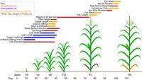
Biologically relevant environmental indices show a clear transition from the vegetative to the reproductive stage of maize. Each line segment represents the environmental index chosen for the labeled trait; the line's color represents the environmental variable(s) used to construct the environmental index and its position on the x-axis represents the time window. The key shows environmental variable types and the number of times each was chosen. An example of maize development is shown; exact developmental timings differ by genotype and environment. (Temp) Temperature, (Precip) precipitation.
The indices chosen by CERIS are also reflected in the principal components analysis (PCA) of the scaled and centered environmental means for each trait (Supplemental Fig. S1). Traits for which CERIS identified similar environmental indices tend to cluster together (e.g., days to anthesis [DTA] and days to silking [DTS]), whereas the weight of 20 kernels (T20KW) was a notable outlier in PCA and had a distinct environmental index from other traits in CERIS (Fig. 1; Supplemental Fig. S1). The identification of similar patterns by different methods, whether considering all traits together without environmental information (PCA) or considering each trait separately while incorporating environmental data (CERIS), supports the robustness of these indices.
We also examined the specific environmental indices chosen by CERIS for robustness to subsampling in addition to biological relevance. As exemplified by DTA, environmental indices chosen from the full data set were highly correlated with the environmental mean (r = −0.996) (Fig. 2A; Supplemental Fig. S2). To confirm that the chosen environmental indices were robust to the exclusion of different genotypes and environments from the training data, CERIS was conducted for each trait on more than 700 training sets containing different combinations of environments and genotypes (see Methods). In general, the environmental indices chosen by CERIS for a given trait remained largely consistent, and for the example trait DTA, 100% of environmental indices identified by CERIS used photothermal ratio (PTR; equal to GDD divided by day length) (Supplemental Fig. S3) as the environmental variable and included the time window of 31–36 days after planting (Supplemental Fig. S4). This environmental index was also biologically relevant. The chosen window occurs before the earliest observed anthesis in the data set, and the environmental variable PTR captures the effects of both temperature (GDD) and day length, both of which are known to affect maize flowering (Neild and Seeley 1977; Hung et al. 2012b). In addition, PTR has previously been identified as an environmental variable affecting flowering time of a maize diversity panel (Li et al. 2021).
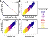
CERIS and prediction results for days to anthesis (DTA). (A) Identified environmental index of photothermal ratio (PTR) measured from 31 to 39 days after planting (DAP) is highly correlated with the observed environmental mean (Obs Env Mean). Representative examples of one-to-two prediction (B), one-to-three prediction (C), and one-to-four prediction (D).
CERIS-chosen environmental indices enable accurate prediction in new environments
The environmental indices identified by CERIS were successfully used for prediction, enabled by the use of the environmental index to connect environments and of genomic relationship to connect genotypes. In brief, the observed phenotype values of each genotype across environments were regressed onto the environmental index values of those environments, generating genotype-specific estimates of intercept and slope values (see Methods). To predict phenotypes in an untested environment (one-to-two scenario, named according to the literature) (Supplemental Fig. S5; Li et al. 2018b; Guo et al. 2020), the slope and intercept values for each genotype were used along with the environmental index value of the new environment (Fig. 2B). To predict untested genotypes in tested environments (one-to-three scenario), genomic prediction was used to predict the slope and intercept values of new genotypes based on the training set of genotypes (Fig. 2C). Finally, these two approaches were combined to predict untested genotypes in untested environments (one-to-four scenario) (Fig. 2D).
Predictions achieved high correlations between observed and predicted values overall (Supplemental Fig. S5), as shown by the example trait DTA (r > 0.93 for all replicates; within-environment prediction accuracies ranged from r = 0.52 to r = 0.88) (representative replicates shown in Figure 2B–D; Supplemental Fig. S6). Flowering time (both DTA and DTS) had the highest prediction accuracy, and prediction accuracy up to 0.74 was achieved for other traits (Supplemental Fig. S5). As expected, prediction in the most difficult scenario (untested genotypes in untested environments, one-to-four) had the lowest prediction accuracy for each trait (Supplemental Fig. S5). These results align with expectations based on previous literature for the number of observed environments required to achieve accurate estimates (Supplemental Fig. S7; Supplemental Methods; Guo et al. 2024).
GWAS of intercept and slope identifies candidate genes for all 19 traits
The CERIS-identified environmental indices were used to plot reaction norms for each trait (Supplemental Fig. S8). Based on these reaction norms, we conducted GWAS (see Methods) to identify loci significantly associated with the intercept (quantifying genotypic mean) and slope (quantifying plasticity with respect to the environmental index). Markers significantly associated with intercept, slope, or both were detected by GWAS for all traits (Supplemental Fig. S9; Supplemental Table S3). In the majority of traits (12 out of 19), GWAS detected a larger number of significant markers (Supplemental Table S3) for a given trait's intercept than for its slope, with notable exceptions found, for example, in DTA and DTS, in which more than five times as many significant markers were detected for slope as for intercept. In addition, the −log10(P)-values of markers obtained from slope and intercept GWASs were themselves significantly (P < 0.00001) positively correlated for each trait, albeit with relatively low correlation coefficients (r = 0.02 to r = 0.21) (Supplemental Fig. S9).
Moving from markers to genes, genes located within 20 kb windows surrounding significant markers were denoted as candidate genes (Supplemental Methods; Kusmec et al. 2017). The number of candidate genes identified for each trait for intercept ranged from zero (EM and TKW) to 434 (tassel branch number [TPBN]) and for slope from zero (EM, KN, and cob diameter [CD], length [CL], and mass [CM]) to 762 (DTS) (Fig. 3; Supplemental Table S4). Up to 16% of the candidate genes detected for slope were also detected for intercept (TPBN), and up to 21% of the genes detected for intercept were also detected for slope (DTS) (Fig. 3; Supplemental Table S4). The pattern of relative proportions of candidate genes for slope and intercept remained generally consistent across the alternative window sizes examined (4 kb to 250 kb) (Supplemental Fig. S10).
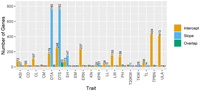
The number of candidate genes for each trait shows the varying genetic architectures of plasticity across traits. Candidate genes were identified as those within a 20 kb window surrounding each significant marker. All genes identified for intercept are shown in orange, all identified for slope are shown in blue, and the genes found in both the slope and intercept GWASs are shown in green.
We conducted Gene Ontology (GO) term enrichment on genes detected by GWAS and found that candidate genes detected for slope had distinct GO term enrichment patterns from those detected for intercept; no term detected as enriched for slope was also detected for intercept, and vice versa (Supplemental Table S5). Enriched GO terms for slope included ATPase-coupled intramembrane lipid transporter activity (all traits) and RNA-directed 5′-3′ RNA polymerase activity (flowering time traits). Six GO terms, including plant hormone signal transduction, were identified as significantly enriched for intercept, all of which were found to be enriched both for plant architecture traits and for all traits (Supplemental Table S5).
GWAS identifies roles in flowering time plasticity for candidate genes
GWAS results for the well-studied flowering time trait DTA (e.g., Buckler et al. 2009; Yang et al. 2013; Li et al. 2016) were examined to validate our model and to identify candidate genes influencing mean flowering time, its plasticity, or both. To identify a subset of these potential candidate genes for DTA to describe in further detail (hereafter, “selected candidate genes”), we examined GO terms and previous literature for genes within 20 kb of significant markers from DTA slope and intercept GWASs. These identified genes included the known flowering genes cct103 and pebp8 for intercept, conz1 and cry3 for slope, and cct1 for both intercept and slope (Fig. 4). Major indel-based haplotypes of each gene from the 26 NAM founder assemblies were identified using BRIDGEcereal (Supplemental Figs. S11–S13; Zhang et al. 2023).
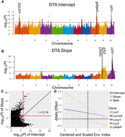
GWAS results for DTA. Manhattan plots of DTA intercept (genotypic mean; A) and slope GWAS (B) results with selected candidate genes labeled. Red lines indicate the SimpleM significance threshold (α = 0.05). (C) The −log10(P)-values of genome-wide markers from GWAS of DTA slope versus intercept. (D) Allelic effects of selected candidate genes identified for the DTA intercept, slope, or both across environmental index values.
A significant SNP in DTA intercept GWAS (Fig. 4A) was located 89 bp downstream from CO CO-LIKE TIMING OF CAB1 protein domain103 (cct103; Zm00001eb023220), which is annotated with GO terms including flower development, regulation of flower development, and regulation of reproductive process (Tello-Ruiz et al. 2016; Törönen et al. 2018). In addition, the ZmCCT gene family in maize to which this gene belongs is known to influence photoperiod sensitivity and days to flowering (Hung et al. 2012b; Yang et al. 2013; Dong et al. 2021). The gene phosphatidylethanolamine-binding protein8 (pebp8; Zm00001eb353250, also called ZCN8; 10 kb downstream from the nearest significant SNP) encodes a florigen and underlies the known flowering time QTL vgt2 (Meng et al. 2011; Bouchet et al. 2013; Guo et al. 2018). Differential expression of pebp8 is associated with differential flowering time (Guo et al. 2018), and alternative indel-based haplotypes upstream of this gene were associated with a significant (P = 0.03) change in DTA intercept among the NAM founders (Supplemental Fig. S11). Associated GO terms include “photoperiodism, flowering” and “regulation of flower development.” This gene has previously been detected as significantly associated with flowering time slope in a diverse maize population (Li et al. 2021).
In the case of DTA slope (Fig. 4B), a significant SNP is located within the first exon of constans1 (conz1; Zm00001eb380460), a gene associated with the GO terms for regulation of flower development and both positive and negative regulation of short-day photoperiodism flowering (Tello-Ruiz et al. 2016; Törönen et al. 2018). It is homologous to the photoperiod genes CONSTANS in Arabidopsis and Heading date1 in rice, shows distinct expression patterns in long and short days (Miller et al. 2008), and promotes flowering in long-day conditions (Bendix et al. 2013). This gene has previously been identified as associated with flowering time slope based on CERIS in another diverse maize population (Li et al. 2021) and is another member of the ZmCCT family (Dong et al. 2021). Another significant SNP is located within the third exon of the gene cryptochrome3 (cry3; Zm00001eb382070). Cryptochromes are a group of photoreceptors that mediate plant responses to both blue and UV light and thereby play a role in floral initiation (Liu et al. 2013; Li et al. 2018a; Vanderstraeten et al. 2018; Dong et al. 2020). In maize, cry3 is sharply downregulated in the seedling leaf proteome after 12 h of light treatment (Gao et al. 2020) and is involved in the blue-light-triggered circadian rhythm pathway that regulates flowering (Li et al. 2018a). This gene is annotated with GO terms, including “long-day photoperiodism, flowering” and “regulation of photoperiodism, flowering, and flower development” (Tello-Ruiz et al. 2016; Törönen et al. 2018). In addition, an insertion located in the second exon of cry3 was significantly correlated (P = 0.00014) with steeper DTA slope among the NAM founders (Supplemental Fig. S12), suggesting a potential causal locus for future study.
Finally, CO CO-LIKE TIMING OF CAB1 protein domain1 (cct1; Zm00001eb418700, also called ZmCCT) is significantly associated with both DTA intercept and slope (Fig. 4). The nearest significant marker in the case of intercept was ∼20 kb upstream of cct1 and, in the case of slope, was within the intron of cct1. This gene is another member of the ZmCCT family (Hung et al. 2012b; Yang et al. 2013; Dong et al. 2021) that is known to have a major effect on photoperiod response and, therefore, flowering time in maize. In a known allele, a CACTA-like transposon within the promoter of cct1 represses cct1 expression and thereby decreases photoperiod sensitivity and reduces flowering time; this allele was important in maize domestication (Hung et al. 2012b; Yang et al. 2013). This is reflected in the significant association of this insertion with DTA intercept (P = 0.046) and slope (P = 0.0017) among the NAM founders (Supplemental Fig. S13). BRIDGEcereal also identified a potential new weak allele of cct1 in Ky21, resulting from an 0.8 kb insertion upstream of the gene rather than the CACTA-like insertion (Supplemental Fig. S13). In addition, cct1 has previously been detected in GWAS of flowering time slope using the CERIS methodology in another maize population (Li et al. 2021). Although cct1 was the only selected candidate gene identified by both DTA intercept and slope GWASs, a total of 83 markers were identified as significant for both DTA intercept and slope (Supplemental Table S3), and the −log10(P)-values of markers from intercept and slope GWASs were significantly positively correlated (r = 0.14, P < 0.00001) (Fig. 4C); together, this indicates that additional loci influencing both intercept and slope are likely present.
To corroborate the results of GWASs on slope and intercept parameters, GWAS was conducted within each environment for each trait. The allelic effect estimates of the selected candidate genes obtained from GWAS within each environment were then regressed on the environmental index (Fig. 4D). The genes identified by only slope GWAS have steep slopes and intercept values near zero, whereas those detected by only intercept GWAS have relatively flat slopes and larger intercept values. Finally, the candidate gene detected by both GWASs (cct1) had both the steepest slope and the largest intercept value among the selected candidate genes investigated (Fig. 4D).
Conceptual understanding of phenotypic plasticity
We constructed a conceptual figure examining two example traits to synthesize our understanding of phenotypic plasticity (Fig. 5). The columns of this figure show the connection between reaction norm diagrams, crossover interactions, and genotypic means (left column); estimated genotype-specific intercepts and slopes (middle column); and, finally, GWAS results for all markers (right column). The two cases depicted are examples of the two extremes of a continuum of genetic architectures, representing the two theories of phenotypic plasticity: the regulatory gene model at one end and the allelic sensitivity model at the other (Fig. 5).
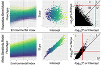
Conceptual visualization of two extreme cases along a continuum of genetic architecture of phenotypic plasticity: examples of a trait entirely following the regulatory gene model (top) and allelic sensitivity model (bottom) of phenotypic plasticity. (Left column) Reaction norms of phenotype across the environmental index; each line represents a single genotype, colored by genotypic mean (intercept). Dashed line indicates where the genotypic mean (intercept) is measured: the mean environmental index value across observed environments. (Middle column) Slope versus intercept values from these reaction norms; each point represents a single genotype, colored by genotypic mean (intercept). (Right column) −log10(P)-values from GWAS of slope (y-axis) and intercept (x-axis). Red lines show GWAS significance threshold, and the black line is x = y; quadrants I–IV are labeled.
In the case exemplifying the regulatory gene model, in which trait mean and its plasticity are entirely controlled by different genes, the intercept and slope of the reaction norm will therefore be uncorrelated. As a result, there will be many crossover interactions, such that the ranking of genotypes will differ across environments. Finally, examining GWAS results of slope versus intercept for such a trait will show significant markers only in quadrants II (significant for slope only) and IV (significant for intercept only), with a complete absence of markers from quadrant I (significant for both intercept and slope).
In contrast, the allelic sensitivity model represents the other end of the continuum of potential genetic architectures, in which trait mean and plasticity are entirely controlled by the same genes. In this case, the intercept and slope of the reaction norm will be highly correlated. This correlation may be positive or negative. In the example of positive correlation shown here, crossover interactions will be rare, and the best genotype is likely to remain constant across environments. Regardless of the direction of correlation between slope and intercept, GWAS results will show a strong correlation between −log10(P)-values for slope and for intercept. However, even in this extreme case of allelic sensitivity, GWAS results will still include many significant markers in quadrants II and IV in addition to those present in quadrant I as expected. Therefore, even in a trait controlled solely by allelic sensitivity, focusing only on significant GWAS results may provide apparent support for the regulatory gene model. This result emphasizes the importance of examining genome-wide patterns to obtain a full picture of the balance between these competing models of phenotypic plasticity in a given scenario.
It is reasonable to state that the regulatory gene model and the allelic sensitivity model describe two extremes along a continuum of possible genetic architectures of phenotypic plasticity, ranging from no overlap between genes controlling trait intercept and slope in the regulatory gene model to complete overlap in the extreme case of the allelic sensitivity model. Many traits may not fall into either extreme and, instead, may have an intermediate genetic architecture within this continuum, with some genes influencing both intercept and slope (allelic sensitivity model), whereas others affect only one of the two (regulatory gene model). The balance between the two extremes may vary across traits, environments, or species. In this study, we have systematically examined phenotypic plasticity in a wide variety of maize traits and found evidence of both models of plasticity at work to varying degrees (Figs. 3, 4; Supplemental Figs. S9, S10; Supplemental Tables S3, S4).
Discussion
Applying CERIS to the maize NAM population enabled the reinstatement of the environmental dimension in both GWAS and genomic prediction, allowing a systematic identification of both environmental and genetic controls of plastic phenotypes in maize. This inventory, available as a track on the MaizeGDB genome browser, forms a community resource and provides context for further dissection of plastic traits in maize. Of course, the experienced environments and plastic responses of crops are complex, integrating many environmental variables and including nonlinear responses (Klingenberg 2019). Although CERIS does not attempt to include all of these factors and instead focuses on linear plasticity in response to a single environmental index per trait (Guo et al. 2024), this method successfully identified major patterns of environmental response and demonstrated that a single influential environmental index is sufficient to achieve high prediction accuracies through genomic prediction (Fig. 2; Supplemental Figs. S5, S6) and to detect loci responding to the chosen index through GWAS (Fig. 4). By enabling both biological understanding and prediction, CERIS combines the advantages of a traditional joint regression analysis with those of a data-driven pattern detection process based on the phenotypic and environmental data. However, in cases in which a single environmental index does not adequately capture the variation of environmental mean, attempts can be made with a composite index from the combination of multiple environmental variables and periods (Piepho 2022), and its biological interpretation should be examined.
CERIS-identified environmental indices enabled biological understanding through detection of markers significantly associated with trait plasticity with respect to the index (slope), the genetic mean for the trait (intercept), or both for all traits examined, as well as corresponding candidate genes. Some markers and candidate genes were detected for either intercept or slope only as expected under the regulatory gene model, whereas others were detected for both slope and intercept as expected under the allelic sensitivity model. Taking the well-studied flowering trait DTA as an example, genes including cct103 and pebp8 were detected for intercept, conz1 and cry3 were detected for slope, and cct1 was detected for both slope and intercept (Fig. 4). As expected, when examining the allelic effects of these selected genes across the environmental gradient, genes identified for slope only tended to have steeper slopes and intercept values nearer zero than those identified for intercept only, whereas cct1 had both a steep slope and a large intercept value and was identified for both slope and intercept (Fig. 4D).
The candidate gene lists for slope also had characteristic differences from those for intercept. In 12 out of the 19 traits, more candidate genes were detected for intercept than for slope using 20 kb windows, indicating that the plasticity of a given trait in maize may often be less polygenic than is the trait per se. However, this pattern varied across traits; for example, more than three times as many candidate genes were detected for slope than for intercept in both DTA and DTS (Fig. 3; Supplemental Fig. S10).
This study provides evidence that both the regulatory gene model and the allelic sensitivity model, which may be viewed as two extremes bounding a continuum of genetic architectures, are important in maize in different contexts. In the case of the regulatory gene model, among the 13 traits for which at least one candidate gene was found by GWAS for both slope and intercept using 20 kb windows, only four traits had any overlap between candidate genes for intercept and for slope. Excluding cct1, the selected candidate genes for the example trait DTA were detected only by slope or only by intercept GWAS, not both. Distinct GO terms were found to be enriched among the candidate genes for intercept as opposed to those for slope. Finally, although all correlations between slope and intercept −log10(P)-values for a given trait were positive, this correlation was as low as 0.02 in the case of LL. However, evidence was also found for the allelic sensitivity model. Up to 21% of all genes detected for a given trait's intercept were also identified for the same trait's slope, as seen in the trait DTS. The known flowering time gene cct1 was found to significantly affect both slope and intercept of DTA, and the gene pebp8 that had previously been identified for DTA slope in another maize panel (Li et al. 2021) was here found to also be associated with DTA intercept. In addition, −log10(P)-values of all genome-wide markers from slope and intercept GWASs were positively correlated for all traits (up to r = 0.21 for TKW), indicating that throughout the genome, significant association with genotypic mean is correlated with significant association with trait plasticity and vice versa. These results suggest that the allelic sensitivity gene model may be more important in some traits (e.g., DTS, DTA), whereas the regulatory gene model may be more important in others (e.g., LL, T20KW).
This result indicates a larger role for the allelic sensitivity model than previous analysis of this population (Kusmec et al. 2017). This larger role may have been detected for allelic sensitivity because the current study takes advantage of the recent development of high-density (more than 20 million) marker data for this population, enabling higher resolution than previous analyses, and examined not only GWAS hits but also genome-wide markers. Although examples of both the regulatory gene and allelic sensitivity models can be found among the significant markers identified by GWAS and their associated candidate genes, the consistent trend of positive correlation between P-values from slope and intercept GWASs uncovered by considering all markers (Fig. 4C; Supplemental Fig. S9) indicates a genetic relationship between mean and plasticity on a genome-wide scale. In fact, this result, showing increased support for the allelic sensitivity model in the whole-genome results compared with when examining only significant markers or candidate genes, is expected (Fig. 5).
Therefore, increasing resolution and power may enable detection of plastic effects of genes previously known to affect genotypic means and vice versa, providing increasing evidence for the allelic sensitivity model. For example, in this study, pebp8 was detected as significantly associated with DTA intercept, whereas it had previously been detected for DTA slope in another maize population (Li et al. 2021). Although the results from each study alone appear to reflect the regulatory gene model, considering both together indicates that the allelic sensitivity model may be more accurate for the effects of pebp8 on maize flowering time. This also agrees with the omnigenic model, which states that all genes expressed in relevant tissues may affect the final phenotype, implying that almost all genes affect almost all phenotypes (Boyle et al. 2017; Liu et al. 2019), which would include both slope and intercept traits. It is also reminiscent of the “missing heritability” debate, in which significant GWAS markers were found to explain only a small proportion of heritability (Manolio et al. 2009), but considering all available markers simultaneously (including those with effects too small to pass significance tests) increased the proportion of heritability explained (Yang et al. 2010). Therefore, further studies may be expected to uncover even more cases of the allelic sensitivity model.
In the face of climate change, continued research on phenotypic plasticity will be crucial. In cases in which the true genetic architecture of plasticity is more similar to that described by the allelic sensitivity model, breeders and growers may have to compromise between genotypic mean and plasticity, whereas cases more similar to the regulatory gene model would enable selecting for these qualities independently. Additionally, phenotypic plasticity plays an important role in evolution of wild species, suggesting that it may also be an important origin of diversity for breeding in domestic species. In “plasticity first evolution,” changes in the environment give rise to a new phenotype via plasticity. Selection then acts on this new phenotype as well as on the degree of plasticity. Finally, if the new phenotype improves fitness in the current environment, it may become canalized in the population (Waddington 1942; Sommer 2020). In domestic species, artificial rather than natural selection may act on these phenotypes, creating the analogous “plasticity first breeding.”
The CERIS process has enabled the identification of highly influential environmental indices calculated from biologically relevant environmental data. This framework allows accurate prediction, even of untested genotypes in untested environments, and the identification of genes responding to these specific environmental conditions. This comprehensive catalog of important environmental and genetic factors underlying plastic traits in maize will provide a valuable resource for the maize community. In turn, our results from a wide variety of traits provide evidence that both the allelic sensitivity model and regulatory genetic model explain phenotypic plasticity in maize, depending on the context. Different traits in the same population show different degrees of overlap between genes controlling slope and intercept, underscoring the need to consider multiple traits before drawing general conclusions about the genetic architecture of plasticity. These insights enabled the creation of conceptual figures illustrating the relationships among important parameters under alternative models for phenotypic plasticity. Additionally, as expected, more support was detected for the allelic sensitivity model when considering all genomic markers rather than only significant GWAS results, highlighting the importance of considering genome-wide markers and increasing mapping power and marker density to better capture the gene–environment interplay. A better understanding of the molecular, environmental, and developmental mechanisms underlying genotype-by-environment interaction will only become more crucial as breeders face the challenge of breeding adapted crops in a changing climate. We encourage application of this systematic approach to other phenotypes and species in order to broaden our understanding of the determinants of phenotypic plasticity.
Methods
Maize NAM and phenotypic data
Previously published (Hung et al. 2012a,b) phenotypic data for 19 traits (Supplemental Table S1) were downloaded from Panzea for the maize NAM population (files “Hung_etal_2012_PNAS_data-120523.zip” and “Hung_etal_2012_Heredity_data-110913.zip”). The maize NAM population consists of 25 families of 200 recombinant inbred lines (RILs) each. To create this population, 25 diverse inbred lines (founders) were each crossed with the common parent B73 and selfed to produce F2 populations, from which RILs were derived (Yu et al. 2008; McMullen et al. 2009). In brief, the 5000 RILs of the maize NAM population were grown in 11 environments spanning six locations over 2 years (Supplemental Fig. S14). In each location, the RILs were planted in a set design, in which each set included all RILs from one NAM family. Within each set were incomplete blocks made up of 20 RILs, B73, and the other parent of the family. Positions of sets, blocks, and lines within blocks were randomized in each environment (Hung et al. 2012a,b).
Outliers were removed following published procedure (Kusmec et al. 2017). Specifically, the interquartile range (IQR) was calculated for each RIL × phenotype combination and for each environment × phenotype combination. Then, any observation that was more than 1.5 × IQR above the third quartile or below the first quartile was removed.
For each trait in each environment, best linear unbiased estimates (BLUEs) were calculated in the lme4 package (Bates et al. 2015) in R (R Core Team 2022) using the following model based on the method of Hung et al. (2012a): where Yijklmnop is a single observation, familyi is the fixed effect of the ith family, RIL(family)ij is the fixed effect of the jth RIL in the ith family, fieldk is the random effect of the kth field, rep(field)kl is the random effect of the lth rep in the kth field, set(rep × field)klm is the random effect of the mth set in the lth rep in the kth field, block(set × rep × field)klmn is the random effect of the nth block in the mth set in the lth rep in the kth field, row(rep × field)klo is the random effect of the oth row in the lth rep in the kth field, column(rep × field)klp is the random effect of the pth column in the lth rep in the kth field, and
  is the random error for a single observation.
Across-environment heritabilities for these data were previously published (Hung et al. 2012a). Within-environment heritability was calculated on an individual plot basis ( ) for each trait (Supplemental Table S6). In our data, across-environment heritability was not significantly correlated with degree of plasticity (calculated as
the environmental mean range divided by the minimum environmental mean per the method of Tonsor et al. 2013) (Supplemental Fig. S15).
) for each trait (Supplemental Table S6). In our data, across-environment heritability was not significantly correlated with degree of plasticity (calculated as
the environmental mean range divided by the minimum environmental mean per the method of Tonsor et al. 2013) (Supplemental Fig. S15).
Genotypic data
For genomic prediction, imputed genotyping-by-sequencing (GBS) data for 955,690 SNPs were downloaded from Panzea (file “ZeaGBSv27_publicSamples_imputedV5_AGPv4-181023.vcf”). Consensus sequences for accessions with more than one entry were calculated with a custom R script. The data were filtered to remove accessions with a missing data rate >60%, SNPs with call rate <70%, and SNPs with minor allele frequencies below 0.01, resulting in a final SNP set of 310,068 markers for 4780 accessions.
For GWAS, SNP and SV data for a total of 20,541,858 markers were obtained from the CyVerse data commons (“NAM_genome_and_annotation_Jan2021_release”). These high-density marker data were generated from a recent de novo genome sequencing of the NAM founders (Hufford et al. 2021). Markers were filtered to remove those with minor allele frequencies below 0.01, leaving a total of 20,357,783 markers.
Environmental data
Environmental variables considered by CERIS included temperature, day length, and combinations of these (Supplemental Fig. S3). In this project, variables including the effects of moisture were also added to the search space for CERIS, as this was found to increase prediction accuracy (Fig. 1; Supplemental Fig. S16). Daily temperature and precipitation data were downloaded from the National Oceanic and Atmospheric Administration (NOAA) website (https://www.ncei.noaa.gov/pub/data/ghcn/daily/by_year/). For each environment, daily values for maximum and minimum temperatures (Tmax and Tmin, respectively) and for precipitation (precip) were calculated as the mean of these values from up to six of the nearest NOAA Global Historical Climatology Network (GHCN) monitors (within 50 km of the location). Potential evapotranspiration (PET) data were downloaded from the U.S. Geological Survey Famine Early Warning Systems Network Data Portal (earlywarning.usgs.gov/fews/product/81) using the “daily data (year)” option and extracted using a custom R script.
Day length (DL) was calculated using the daylength() function in the geosphere package in R. Water balance was calculated as precipitation − PET. Other environmental variables were calculated as previously described (Li et al. 2018b, 2021, 2022; Guo et al. 2020; Mu et al. 2022). Specifically, GDDs were calculated according to method 2 described by McMaster and Wilhelm (1997). Photothermal time (PTT) was calculated as GDD × DL, photothermal ratio (PTR) as GDD/DL, photothermal difference 1 (PTD1) as (Tmax – Tmin) × DL, photothermal difference 2 (PTD2) as (Tmax – Tmin)/DL, PTS as (Tmax2 – Tmin2) × DL2, and diurnal temperature range (DTR) as (Tmax – Tmin).
CERIS
CERIS was conducted to identify environmental indices as previously described (Li et al. 2018b, 2021, 2022; Guo et al. 2020; Mu et al. 2022). By design, CERIS aims to capture the single most influential time window across environments. Although this approach of choosing a single, fixed day-based window means that the exact growth stage during the CERIS window will vary by both genotype and environment, this model has been found to be useful and is frequently used (Li et al. 2018b, 2022; Mu et al. 2022; Guo et al. 2024). In brief, the environmental mean for each trait in each environment was the mean of the phenotype BLUEs observed in that environment, using data from accessions phenotyped in at least three environments. Then, the average value of each of the 11 potential environmental variables was calculated for each environment for all windows DAPi to DAPj, where DAPx is x days after planting and 5 < (j – i) < 60. Each trait was categorized as either a flowering time or harvest trait depending on when it was measured; search windows for each category were limited to those that concluded before the trait was measured (Supplemental Table S1). The window × environmental covariate combination with the highest correlation with the environmental mean was selected as the environmental index. CERIS was conducted on each training set for prediction as well as on the full data set.
Performance prediction
For each trait, the following random regression model based on the method of Ly et al. (2018) was fit in ASReml 4.1:
 where y is the BLUE value for a particular accession in a given environment; μ is the overall mean; xE is the vector of the CERIS-identified environmental index value in each environment, centered on zero and scaled to have
a variance of one; β is the fixed regression coefficient with respect to the environmental index; uG is the vector of genotypic means (intercepts), uG ∼ N(0,
where y is the BLUE value for a particular accession in a given environment; μ is the overall mean; xE is the vector of the CERIS-identified environmental index value in each environment, centered on zero and scaled to have
a variance of one; β is the fixed regression coefficient with respect to the environmental index; uG is the vector of genotypic means (intercepts), uG ∼ N(0,  K), where K is the genomic relationship matrix; bG is the vector of the plasticities (slopes) in response to the environmental index values xE, bG ∼ N(0,
  K); e is a vector of residuals with environment-specific variance; ZG is the incidence matrix for the effects uG and bG; ZE is the incidence matrix for the environmental index values xE; ○ is the Hadamard product; σGB is the covariance between uG and bG; nE is the number of environments; nG is the number of observed genotypes, and I is the identity matrix.
Prediction scenarios were named based on the literature (Li et al. 2018b; Guo et al. 2020) as diagrammed in Supplemental Figure S5, in which “one” represents tested genotypes in tested environments (the training set); “two,” tested genotypes in untested environments; “three,” untested genotypes in tested environments; and, finally, “four,” untested genotypes in untested environments. For one-to-two prediction, data from nE − 1 environments were used as the training set to predict the other environment; this was repeated until all environments were predicted. For one-to-three prediction, 50% of the genotypes from each family were used as the training set and used to predict the other 50% of genotypes (twofold cross-validation). In one-to-four prediction, 50% of genotypes in each family (twofold cross-validation for genotypes) in nE − 1 environments were used as the training set to predict the other 50% of genotypes in the remaining environment. One-to-three and one-to-four predictions were repeated for 30 random replicates. In all prediction scenarios, CERIS was run on each training set to identify the environmental index used for that prediction. Genomic prediction for intercept and slope was conducted within families to improve computational speed by reducing the sizes of the matrices to be calculated and manipulated (with our computing resources, this reduced computing time from ∼17 h for the full NAM population per trait to ∼1 min per family per trait).
GWAS
MLM-based GWAS was conducted in GCTA v1.91.2beta using the ‐‐mlma option (Yang et al. 2011). MLM GWAS was chosen rather than biparental or other approaches because the maize NAM panel was designed to exploit both linkage information during RIL development and LD among NAM founders (Yu et al. 2008; Gage et al. 2020), and GWAS leverages this full NAM design in a way biparental approaches do not. GWAS has therefore been used extensively and successfully in this panel (Hung et al. 2012b; Hufford et al. 2021).
To correct for multiple testing, the significance threshold was calculated by the SimpleM method (α = 0.05) (Gao et al. 2008). To avoid the overshrinkage caused by using the kinship matrix in both the estimation of the intercept (uG) and slope (bG) as well as in GWAS, a fixed linear model regressing phenotypes onto the environmental index was used to estimate the intercept and slope for use in GWAS (Piepho et al. 2012). For each trait, then, GWASs were conducted for the trait's intercept and slope estimated from the full data set as well as on trait BLUEs in each environment, for a total of up to 13 GWASs per trait. The correlation between the −log10(P)-values of markers from slope and intercept GWASs for each trait was examined to assess whether or not the significance level for trait mean was positively correlated with the significance for trait plasticity at the marker level. Our goal here was to identify markers with similar evidence (particularly, significant evidence) of association with both the intercept and slope of a given trait, regardless of effect size. As such, we were primarily interested in markers with similar evidence for effect (measured by P-values) versus similar effect sizes (allelic effects).
To identify candidate genes for a given trait from GWAS, the full list of genes and their coordinates in the Zm-B73-REFERENCE-NAM-5.0 genome assembly were downloaded from MaizeGDB (see Supplemental Methods; https://download.maizegdb.org/Zm-B73-REFERENCE-NAM-5.0/, file name “Zm-B73-REFERENCE-NAM-5.0_Zm00001eb.1.gff3.gz”). All genes within a set distance of significant marker(s) were saved as candidate genes for that trait. Results were compiled for 13 window sizes (4 kb, 10 kb, 20 kb, 30 kb, 40 kb, 60 kb, 80 kb, 100 kb, 150 kb, 200 kb, and 250 kb; these correspond to average LD [r2] of 0.19, 0.18, 0.16, 0.15, 0.14, 0.13, 0.12, 0.11, 0.10, 0.095, and 0.091, respectively); windows were centered around each significant marker.
To identify significantly enriched GO terms, lists of genes within 20 kb windows centered on significant markers (candidate genes) were analyzed with g:Profiler version e106_eg53_p16_65fcd97 with g:SCS multiple testing correction (Raudvere et al. 2019). This analysis was conducted with the candidate gene lists from both slope and intercept GWASs for all traits combined as well as for each of the three types of traits (flowering time, plant architecture, and yield). To identify a subset of candidate genes as selected candidate genes for further discussion and Manhattan plot annotation, GO terms were downloaded from Gramene BioMart (Tello-Ruiz et al. 2016; Törönen et al. 2018; https://ensembl.gramene.org/biomart/martview) and examined for genes of interest within 20 kb of significant markers. Allelic effects from environment-specific GWAS of the most significant marker within each selected candidate gene were regressed on the environmental index to visualize allelic effects of genes across the environmental gradient. Genetic nomenclature was obtained from MaizeGDB (Woodhouse et al. 2021). Major haplotypes based on large indels were found using BRIDGEcereal (Supplemental Methods; Zhang et al. 2023).
Data access
GWAS results are deposited as a track in the genome browser at MaizeGDB (https://jbrowse.maizegdb.org/?data=B73&loc=chr9%3A1..163004744&tracks=gene_models_official%2CTibbs-Cortes2024). Scripts are deposited at GitHub (https://github.com/LTibbs/MaizeNAMplasticity) and available as Supplemental Code. CERIS was implemented based on code from GitHub (https://github.com/jmyu/CERIS_JGRA).
Competing interest statement
The authors declare no competing interests.
Acknowledgments
This research was supported by the Agriculture and Food Research Initiative competitive grant (2021-67013-33833) and the Hatch project (1021013) from the United States Department of Agriculture (USDA) National Institute of Food and Agriculture, the National Science Foundation (OIA-2121410), the Iowa State University Plant Sciences Institute, the Iowa State University Raymond F. Baker Center for Plant Breeding, and the USDA Agricultural Research Service In-House Projects (2090-21000-039-00D and 5030-21000-072-00-D). L.E.T.-C. was supported by the National Science Foundation Graduate Research Fellowship Program (grant no. 1744592) and a postdoctoral fellowship funded by the USDA Agricultural Research Service SCINet Program and AI Center of Excellence, ARS project numbers 0201-88888-003-000D and 0201-88888-002-000D. Mention of trade names or commercial products in this publication is solely for the purpose of providing specific information and does not imply recommendation or endorsement by the U.S. Department of Agriculture. USDA is an equal opportunity provider and employer.
Author contributions: L.E.T.-C. contributed conceptualization, data curation, formal analysis, investigation, methodology, software, visualization, writing of the original draft, and reviewing and editing. T.G. contributed methodology and reviewing and editing. C.M.A. contributed resources and reviewing and editing. X.L. contributed conceptualization, funding acquisition, methodology, resources, supervision, and reviewing and editing. J.Y. contributed conceptualization, funding acquisition, project administration, resources, supervision, and reviewing and editing.
Footnotes
-
[Supplemental material is available for this article.]
-
Article published online before print. Article, supplemental material, and publication date are at https://www.genome.org/cgi/doi/10.1101/gr.279027.124.
-
Freely available online through the Genome Research Open Access option.
- Received January 24, 2024.
- Accepted August 6, 2024.
This article, published in Genome Research, is available under a Creative Commons License (Attribution-NonCommercial 4.0 International), as described at http://creativecommons.org/licenses/by-nc/4.0/.


