
Rapid SARS-CoV-2 surveillance using clinical, pooled, or wastewater sequence as a sensor for population change
- Apurva Narechania1,2,
- Dean Bobo1,3,
- Kevin Deitz1,
- Rob DeSalle1,
- Paul J. Planet1,4,5 and
- Barun Mathema6
- 1Institute for Comparative Genomics, American Museum of Natural History, New York, New York 10024, USA;
- 2Section for Hologenomics, The Globe Institute, University of Copenhagen, DK-1353 Copenhagen, Denmark;
- 3Department of Ecology, Evolution, and Environmental Biology, Columbia University, New York, New York 10027, USA;
- 4Division of Pediatric Infectious Diseases, Children's Hospital of Philadelphia, Philadelphia, Pennsylvania 19104, USA;
- 5Department of Pediatrics, Perelman College of Medicine, University of Pennsylvania, Philadelphia, Pennsylvania 19104, USA;
- 6Department of Epidemiology, Mailman School of Public Health, Columbia University, New York, New York 10032, USA
Abstract
The COVID-19 pandemic has highlighted the critical role of genomic surveillance for guiding policy and control. Timeliness is key, but sequence alignment and phylogeny slow most surveillance techniques. Millions of SARS-CoV-2 genomes have been assembled. Phylogenetic methods are ill equipped to handle this sheer scale. We introduce a pangenomic measure that examines the information diversity of a k-mer library drawn from a country's complete set of clinical, pooled, or wastewater sequence. Quantifying diversity is central to ecology. Hill numbers, or the effective number of species in a sample, provide a simple metric for comparing species diversity across environments. The more diverse the sample, the higher the Hill number. We adopt this ecological approach and consider each k-mer an individual and each genome a transect in the pangenome of the species. Structured in this way, Hill numbers summarize the temporal trajectory of pandemic variants, collapsing each day's assemblies into genome equivalents. For pooled or wastewater sequence, we instead compare days using survey sequence divorced from individual infections. Across data from the UK, USA, and South Africa, we trace the ascendance of new variants of concern as they emerge in local populations well before these variants are named and added to phylogenetic databases. Using data from San Diego wastewater, we monitor these same population changes from raw, unassembled sequence. This history of emerging variants senses all available data as it is sequenced, intimating variant sweeps to dominance or declines to extinction at the leading edge of the COVID-19 pandemic.
The COVID-19 pandemic has been fueled by the repeated emergence of SARS-CoV-2 variants, a few of which have propelled worldwide, asynchronous waves of infection (Koelle et al. 2022). First arising in late 2019 in Wuhan, China, the spread of the D614G mutation led to sequential waves of variants of concern (VOCs) about 9 months later, significantly broadening the pandemic's reach and challenging concerted efforts at its control (Li et al. 2020). Beta and Gamma variants drove regional resurgences, but Alpha, Delta, and Omicron occurred globally (Dhar et al. 2021; Viana et al. 2022). The advent of each variant led to the near extinction of the population from which it arose (Korber et al. 2020). The architecture of this pandemic is, therefore, marked by periods of transition, tipping a population toward an emerging VOC followed by its near-complete sweep to dominance.
At the pandemic's outset, epidemiological work was focused on transmission networks, but SARS-CoV-2's high rates of infection quickly outstripped our ability to trace it (Li et al. 2020). When it became clear that even focused global efforts would only characterize a fraction of infections, researchers turned to phylodynamic approaches to understand SARS-CoV-2's population structure (Grenfell et al. 2004; Volz et al. 2013; Chiara et al. 2023). Genomics was at the center of this effort. Rapid sequencing and whole genome phylogeny updated in quasi-real time enabled surveillance that was a few weeks to a month behind the edge of the pandemic curve (Gardy and Loman 2018). In a crisis of COVID-19's scale and speed, eliminating this analysis lag can mean the difference between a timely, reasonable public health response and failure to understand and anticipate the disease's next turn.
Phylodynamics is predicated on genetic variation. Without variation, phylogenetic approaches yield star trees with no evolutionary structure. The high mutation rate among pathogens, especially among RNA viruses like SARS-CoV-2, ensures the accumulation of sufficient diversity to reconstruct pathogen evolutionary history even over the relatively short timescales that comprise an outbreak. However, as a genomic surveillance technique, phylodynamics is costly. Tools like Nextstrain align genomes, reconstruct phylogenies, and date internal nodes using Bayesian and likelihood approaches (Hadfield et al. 2018). These techniques are among the most computationally expensive algorithms in bioinformatics. Intractable beyond a few thousand sequences, these phylodynamic approaches must operate on population subsamples, and subsamples are subject to the vagaries of data curation. More recent work in parsimony can scale to hundreds of thousands of genomes (Turakhia et al. 2021) but still requires an existing phylogeny. All phylodynamic approaches are yoked to references and most are ill equipped to respond to evolutionary novelty. We argue that genomic surveillance should herald the appearance of previously unseen variants without having to resort to comparison with assembled and curated genomes. Surveillance is currently hamstrung by the historical bias inherent to marker-based analysis and the wait between variant discovery and a database update. The existing pandemic toolbox, therefore, lacks unbiased approaches to quickly model the population genomics of all sequences available.
We propose a method that summarizes the temporal trajectory of pandemic variants by collapsing each day's assemblies into a single metric. In the case of pooled or wastewater sequence, this same metric is repurposed to measure survey sequence compression across days. Our method does not subsample, align sequences, or build trees. Still, we describe the major arcs of the COVID-19 pandemic. Our inspiration comes from long-standing definitions of diversity used in ecology. We use Hill numbers (Hill 1973; Alberdi and Gilbert 2019), extensions of Shannon's theory of information entropy (Shannon 1948). Rather than using these numbers to compute traditional ecological quantities like the diversity of species in an area, we use them to compute the diversity of genomic information. For example, we envision each unique k-mer a species and each genome a transect sampled from the pangenome. Applying Hill numbers in this way allows us to measure a collection of genomes in terms of genomic equivalents, or a group of sequence pools as the effective number of groups. We show that tracing a pandemic curve with these new metrics enables the use of sequence as a real-time sensor, tracking both the emergence of variants over time and the extent of their spread.
Results
Reframing ecological concepts for pandemic genomics
To measure the information diversity of a population, we use ecological definitions that condense the influence of millions
of genomes or terabases of raw sequence into a single value. In ecology, the effective number of species is a quantity used
to provide an intuitive and simple metric for comparing species diversity across environments. Hill (1973) defined the effective number of species of order q as
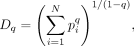 where pi is the frequency of a particular species i, and N is the total number of unique species. The parameter q determines the equation's responsiveness to rare (lower q) or common species (higher q). As q tends toward one, we weigh all species by their frequency regardless of whether they are common or rare, and the limit of
this equation invokes Shannon's concept of generalized information entropy. Among ecologists, information entropy is better
known as the Shannon index which measures the difficulty in predicting the next species observation given a cache of existing
observations. The exponent of the Shannon entropy yields the effective number of species, a quantity commonly referred to
as the Hill number. When q = 1 we have
where pi is the frequency of a particular species i, and N is the total number of unique species. The parameter q determines the equation's responsiveness to rare (lower q) or common species (higher q). As q tends toward one, we weigh all species by their frequency regardless of whether they are common or rare, and the limit of
this equation invokes Shannon's concept of generalized information entropy. Among ecologists, information entropy is better
known as the Shannon index which measures the difficulty in predicting the next species observation given a cache of existing
observations. The exponent of the Shannon entropy yields the effective number of species, a quantity commonly referred to
as the Hill number. When q = 1 we have
Hill numbers are best conceptualized as the number of equally abundant species required to recapitulate the measured diversity in a sample. The more diverse the sample, the higher the Hill number. The Hill number is not unique to ecological analysis. For example, in natural language processing (NLP), this same quantity is termed perplexity, a key measure in the evaluation of language models (Brown et al. 1992).
While species Hill numbers are helpful for understanding the nature of any given sample, ecologists are often interested in
comparisons across samples. The motivation is to assess the experimental design and/or to gauge the piecemeal complexity of
an ecosystem. The beta diversity, a measure of differentiation between all local sites, extends species Hill numbers to Hill
numbers of samples. Ecologists use an effective number of samples to understand the competing effects of their sampling and
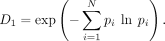
the innate diversity of their transects (Jost 2007; Marcon et al. 2012, 2014). The Hill number based on beta diversity is given as
 an expression that incorporates the Kullback–Leibler divergence (Kullback and Leibler 1951) to yield the effective number of samples. Here, N is the number of unique species, M is the number of samples, psi is the frequency of a particular species i in a particular sample s, pi is the frequency of a particular species i across all samples, and ws weighs all observations in sample s relative to all individuals censused in the experiment.
The effective number of samples measures their compressibility. If the samples share many species and if individuals are evenly distributed across these species, the samples essentially collapse, yielding a lower Hill number. If the samples are highly diverse and the individuals scattered among these divergent species, the effective number of samples approaches M (Fig. 1). This interpretation of the beta diversity relies heavily on information theoretic principles, reflecting the broad and powerful implications of Shannon's original theory of entropy and communication (Shannon 1948). Recent papers have used this concept to measure microbial (Chiu and Chao 2016), viral (Moustafa and Planet 2021), and metagenomic diversity (Ma and Li 2018).
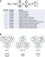
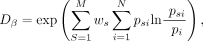
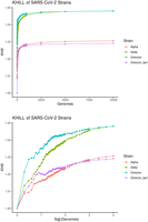
The KHILL metric. We adopt ecological definitions for beta diversity to calculate the effective number of genomes (KHILL) in any set. We explicitly describe the analogy in terms of variables in the KHILL expression (A). Genomes with overlapping k-mer identities and similar k-mer frequencies will tend to have a lower KHILL (B).
In the ecological framework we describe here, the sample functions as a container for observations of species and their frequencies. However, the container can be anything. We reframe these classic ecological equations to operate in a genomic context. Instead of counting species, we count k-mers. Instead of spatial transects, we sample genomes. k-mer approaches abound in the genomics literature, some specifically geared toward viral biodiversity (Cedeño-Pérez and Gómez-Romero 2022; Lebatteux et al. 2022; Thommana et al. 2022). Our approach couches a string-based analysis within the broad strokes of a mathematics designed for ecologies. If the goal in ecology is to generalize to gamma diversity (Whittaker 1960), the genomic analogy is generalizing to the pangenome. This is made explicit in Figure 1.
We aim to use this new method in two ways distinguished by how we define M in Figure 1A. If M is the number of discrete, clinical genomes, the Hill number defines the effective number of genomes, or genome equivalents. If M is the number of days, then the Hill number computes the effective number of days where each day is represented by survey sequence. Pools can be combined at the clinic or gathered downstream in wastewater. Regardless of the nature of M, we term this new quantity KHILL. If we consider a set of identical sequence, KHILL will reduce to 1, whereas in a set of sequence with no information overlap, KHILL will achieve its maximum, the number of groups M considered (Fig. 1B).
Equipped with this new metric of genome information diversity, we can track population dynamics across any axis of change. If the axis is temporal, we calculate KHILLs for each day where M is the number of genomes considered on that day. In Figure 2A, we show a stable community of subtype genomes experiencing a disturbance that signifies the emergence of a new variant. If selection favors this variant, the population will pass through a KHILL peak where genome equivalents find a local maximum. Prior variants coexist in almost equal measure with the newcomer. This local maximum will erode if the new variant sweeps through the population. When prior subtypes are driven to extinction and a single variant pervades, we expect a local minimum for KHILL.
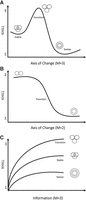
KHILL cartoons. In a population genomic context, KHILL can be used to track changing clinical genomic complexity over time and/or space. We expect that in a pandemic, a VOC will increase the information diversity of a stable population. If this transition is favored, the variant will sweep the population (A). In a pooled or wastewater context, KHILL can function as a measure of compression of unassembled, raw sequence across days, with a drastic change revealing the potential arrival of a new variant (B). Genomes sampled from a transitioning population will exhibit higher KHILL than a population that has settled into a dominant variant (C).
For sequence pools, we instead perform KHILL pairwise comparisons (M = 2) of the most recent day's survey sequence to sequence from all prior days. This type of analysis is similar to autocorrelation, but our metric is KHILL, the information diversity compressed into the effective number of days. If the recent pooled sequence diverges from the past sequence, we expect a bend in the KHILL curve describing a change in sequence compression on the appearance of a new dominant variant. For pairwise comparisons, KHILL will vary between 1 and 2 (Fig. 2B). We mark significant changes in the time course using Bayesian Change Point detection (Barry and Hartigan 1993).
A further application of our approach is to pangenomes, the accrued genomic content of any given species (Tettelin et al. 2005). Because the KHILL metric functions as a measure of genome equivalents independent of functional content, the concept can bring new clarity to pangenome dynamics. The state of the art in pangenomes is wedded to genes and/or alignments. Phylogenomic methods calculate orthologs (Nichio et al. 2017), and pangenome graphs fork alignments along multiple, disparate paths (Eizenga et al. 2020). While a number of these methods have achieved significant speed (Turakhia et al. 2021), KHILL obviates the need for phylogenetics entirely by calculating information theoretic quantities on containers of k-mers. We think not in terms of genes, but in terms of unique strings of information. As we accumulate genomes, the KHILL curve of a transitioning population will asymptote to a higher value than the simpler population left in the wake of a selective sweep (Fig. 2C).
Since the KHILL approach operates on containers of unaligned strings our main computational challenge is to reduce the number of string comparisons without sacrificing sensitivity. A smaller string size requires lower memory, but a larger string size affords higher resolution. For this analysis, we chose a k-mer size of 19 (Ondov et al. 2016), and find that a string sketch (Broder 1998), as adopted in programs like MASH (Ondov et al. 2016), adequately reflects calculations made on the whole population. We need only a fraction of available k-mers to carry each container's signal. Using a bottom-k sketch (Cohen 1997) of hashed strings, we accelerate KHILL calculations by many orders of magnitude. We use MurmurHash (Appleby 2015) to hash our k-mer strings with a sampling rate of 0.01. A deeper sketch may capture more details of the pandemic trajectory, but a very shallow sketch is often enough to outline the main variant transitions. Sketch depth and k-mer size (more detail in the next section) are provided as options to the user looking to negotiate between resolution and computational savings.
Our approach is unusual in that we are not looking for evidence of specific genetic events. With sketched strings of unaligned data, we sacrifice most of the products of modern bioinformatics: the discovery of mapped genome variation like alleles in particular genes, indels in noncoding regions, or genome-scale structural rearrangement. But we gain a fast, intuitive metric that summarizes the contributions of both micro-variation on the mutational scale, and macro-variation such as the presence/absence of genomic elements.
Using KHILL to track emerging SARS-CoV-2 variants of concern
The United Kingdom is a model for COVID-19 genomic surveillance (The COVID-19 Genomics UK (COG-UK) consortium 2020). The COVID-19 Genomics UK consortium has accumulated more genomes and more metadata than any other regional health organization. Figure 3 shows the 7-day moving average of the 22.2 million UK cases reported as of July 15, 2022 (panel A) with spikes coincident with the emergence of the UK's three main VOCs: Alpha, Delta, and Omicron (panel B). Panels A and B rehash the accepted epidemiological approach, case counts augmented by phylogenetic annotation. Using the complete set of 2.5 million UK genomes sequenced from these reported cases, we add panel C, a single KHILL value calculated for each day. With the emergence of each variant, KHILL rises until it reaches a local maximum where sequenced genomes are evenly distributed between the old variant and the new.
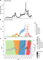
The UK COVID-19 pandemic. We show new case burden (A) and gross phylogenetic classification (B) for the UK pandemic since its inception. The three distinct KHILL peaks signal the arrival of Alpha (November 2020), Delta (May 2021), and Omicron (November 2022) well before each variant's spike in cases (C).
Against a background of the UK's dominant variant waves, these peaks mark clear transitions in the pandemic. Notably, the stark peaks that presage the emergence of Delta and Omicron occur well before each variant's burden of cases. In May 2021, public measures like masking and travel restrictions suppressed new infections, but it is in this month that we observe the KHILL peak signaling the arrival of Delta. The changing complexity of the viral population is reflected in this curve of daily genome equivalents regardless of the volume of cases and regardless of the variant. Because the expression for the effective number of genomes is weighted, days with just tens of sequences scale with days that may have tens of thousands.
In the UK, each population transition—signified by the three KHILL peaks—was harbinger of a selective sweep. A peak's ascent reflects the accumulating momentum of a VOC, while the descent suggests this new variant's dominance. Alpha swept the population in March 2021 (Davies et al. 2021), Delta by July 2021 (Kläser et al. 2022), and Omicron by January 2022 (Paton et al. 2022). In each case, KHILL settles into a local minimum of about 1.03 effective genomes highlighting the near clonality of the new variant in the viral population. Rising KHILL values within the Delta and Omicron waves suggest that we also detect accruing diversity within the Delta (mixing of AY.4, B.1.617.2, and AY.4.2) and Omicron (BA.1 and BA.2) lineages over time. The height of the KHILL peak responds to both the degree of population heterogeneity, and the overall genetic distance between the viral mixture's components. This property is particularly useful in understanding KHILL as a pangenomic measure. Though evidence of evolving subvariants requires a deeper sketch (Supplemental Fig. 1), this within-wave signal tracks the information complexity of steady evolution following a selective sweep.
The height of the peak is also sensitive to k-mer size. In Supplemental Figure 2, we show the Alpha to Delta transition for k-mer sizes ranging from 1 to 31. In each case, we find the transition peak where we expect it, but a k-mer size of at least 15 is needed to assure sufficient amplitude. A k-mer size of 19 achieves a balance between sensitivity and memory savings.
We performed the same type of analysis for both the United States and South African pandemics. Though we see regional differences in terms of which variants were dominant at which times, in almost every case, the KHILL curve tracks the arrival of prevailing variants. Unlike the UK, the start of the U.S. pandemic is variably complex with near-simultaneous transmission events from around the world (Gonzalez-Reiche et al. 2020; Worobey et al. 2020) manifesting as a noisiness in KHILL (Supplemental Fig. 3). The introduction of Alpha flattens this diversity. In South Africa, the Beta variant achieved a higher share of infection than in either the UK or the United States (Tegally et al. 2021). Though sparse South African genomic sampling results in a stochastic KHILL curve, we observe a clear peak demarcating the transition between Delta/Omicron. The transition between Beta and Delta seems bimodal and broad, a result that might have achieved more refinement with denser sampling (Supplemental Fig. 4).
KHILL anticipates new variants before they are named
To illustrate how traditional methods lag in their detection of variant changes in a population, we revisited the UK KHILL curve, focusing on the emergence of BA2. Figure 4A shows the curve overlayed on version 1.2.101 Pangolin annotations. This version was released on January 28, 2022. Before this release, it is already clear that a steady increase in the effective number of genomes is underway, culminating in a peak just a few weeks later. The 1.2.101 Pangolin annotation conflates this additional heterogeneity into a single annotation for B.1.1.529. About 1 month later, in panel B we see that the KHILL trace anticipated the arrival of a new Omicron subvariant, BA2. BA2 entered the lexicon too late to offer useful classification for what was clearly an emerging variant as early as January 1, 2022. The BA2 classification seems to trail the BA2 KHILL peak by a full month and the beginning of the BA2 curve by 2 months. KHILL was picking up something new well before BA2 was fixed into the databases offering an immediacy that phylogenetic, reference-bound, and annotated techniques like Pangolin lack.
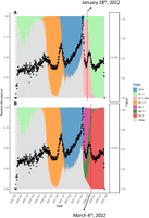
KHILL anticipates new variants. We show that in the UK population, a KHILL peak mounting around January 1, 2022 forecasted the emergence of the new Omicron subvariant, BA2. This variant was not properly classified by Pangolin (A) until 2 months later (B), well after BA2 had saturated the population.
The existence and extent of this lag depend on the responsiveness and efficiency of annotation clearinghouses. In Supplemental Figures 5 and 6, we show that Pangolin was primed for the appearance of both Delta and Omicron. Delta was first detected on October 5, 2020 in India (Dhar et al. 2021). Omicron was first detected on November 22, 2021 in Botswana and South Africa (Viana et al. 2022). These early detections coupled with worldwide urgency motivated quick classification and annotation. These extraordinary efforts met the gravity of the time. However, pandemics unfold at differing rates and sometimes under the public radar. Whether it is BA2, Delta, or Omicron, we show that given sufficient sequence, KHILL responds to the emergence of novelty before or in parallel with vetted classifications.
Tracking the edge of a pandemic with sequence pools and wastewater
Thus far, we have used KHILL to trace the pandemic's natural history. What if instead, we want to ask the simple but important question: Is there anything new in my latest sequence? As the pandemic progressed, surveillance extended beyond the clinic into pooled sequence accumulated in sewage (Valieris et al. 2022). We repurposed KHILL to detect new signal in a sequence stream. Our information diversity approach is not designed to assign novel strains as they emerge in wastewater. But it does detect change.
Sequence dissociated from individual, discrete infections is necessarily unassembled. As a first step, we show that since KHILL relies only on sketched strings, reads alone produce a curve that mirrors the pattern we see for all assemblies. For the curve in Supplemental Figure 7, we simulated 250,000 reads from each genome of a random sample of 100 genomes selected daily over the course of the UK pandemic.
For pandemic policy and infection control, the key question is whether today's reads diverge from yesterday's sequence and whether this divergence is sustained over a week or even a month. In other words, given a cache of past sequence, how quickly can we determine if the population is currently changing? Moreover, can we detect this change without having to annotate and/or characterize the new variant? We generated a sequence stream by simulating reads from each day's genomes over the entire UK pandemic. We joined and shuffled these simulated reads retaining only 400,000 as a kind of daily signature for the overall state of the region. Following the model in Figure 2B, we compared the most recent day's reads to all previous days in pairwise fashion. The conceptual shift here is in the nature of the container. For any given KHILL comparison, we have a survey sequence for 2 days (M = 2). If the most recent reads are information diverse, KHILL will tend toward two. If the reads are instead compressible, KHILL will tend toward one.
We take this approach in Figure 5. A collection of reads from December 1, 2021 shows steady and low KHILL through June 2021, consistent with comparisons of Delta against Delta. The peak in this first panel corresponds to comparisons of Delta against Alpha. Omicron emerged in late 2021. Reads from December 15, 2021 distinguish this new Omicron-tinged set from all the Delta signatures that came before. Reads from January 1, 2022 and January 15, 2022 depart from Delta even further, an indication of something genuinely new. The emergence of a new variant is marked by a clear transition in KHILL values. At least two starkly different populations emerge: days before the new variant appeared and days after (Fig. 5A,B). As the KHILL stream accumulates, shadows of previous variants are also clearly visible. For statistical rigor, we apply Bayesian Change Point analysis to tag significant transitions and note that these detected points correspond to known population dynamics. Notably, posterior probability peaks within the Omicron transition correspond to Omicron subvariants (Fig. 5A).
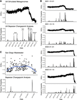
SARS-CoV-2 in raw, pooled sequence. We show pairwise comparisons of the simulated survey sequence from July 11, 2022 to the simulated survey sequence from all prior days during the course of the UK pandemic. This autocorrelation analysis shows a pronounced downward swing marking the turnover from Delta to Omicron. The shadows of previous transitions are also evident in the KHILL trace. We show that these transitions are significant using Bayesian Changepoint Detection and annotate each transition with its emerging variant (A). To demonstrate how this technique can be used in real time, we compare simulated survey sequence from four-time points chosen to track the arrival of Omicron. As Omicron suffuses the population, we can see the KHILL curve plunge with respect to time points dominated by Delta (B). San Diego wastewater data show similar—albeit noisier—transitions between variants. Comparison of raw sequence from a day dominated by Omicron to all prior days shows clear and significant separation between Alpha/Epsilon and Delta/Omicron (C).
Clearly, simulated sequence pools are amenable to KHILL surveillance analysis. But will the technique work for real data? In principle, wastewater is a pool of infections. Changes in wastewater information diversity should expose new variants. In Figure 5C, we show that despite the noise inherent to wastewater data, we discern two clear transitions in the San Diego pandemic (Karthikeyan et al. 2022): the rise of Alpha in January of 2021, and the rise of Omicron that December. Because KHILL measures change in terms of k-mer representation and frequency across days, it is sensitive to uneven coverage and the noise characteristic of metagenomic sequencing in a way that marker-based analysis is not. To screen the noisiest time points and assure even coverage, we calculated the alpha diversity of k-mers sampled from each day and kept only those days within one standard deviation of the mean (Supplemental Fig. 8). This alpha diversity screen tightened our curve significantly, but the emergence of delta, which is known to have dominated San Diego infections by July 2021, remains hidden. Karthikeyan et al. (2022) use references to squash this noise by forcing alignment, but alignment limits the detection of novelty. Given comparable sequence coverage and depth across days, KHILL can eliminate the need for references, quicken the pace of discovery, and capture incipient novelty possibly lost to marker-based analysis. Computing KHILL from pooled or wastewater reads realizes our ambition of making streamed sequence a kind of online sensor (Erlich 2015) that can aggregate signal directly and in real time and the very edge of a pandemic.
Simulation
KHILL is sensitive and capable of monitoring shifts in the viral population despite the handful of changes that distinguish each variant. To better understand the number and type of phenomena we can detect with KHILL, we simulated blocks of change across one hundred 30 kb genomes varying each population from one base to 500 contiguous bases across several classes of mutation, including insertion, deletion, duplication, and transposition (Supplemental Fig. 9; Rice et al. 2000). For SARS-CoV-2, mutation blocks of 1–5 bases are biologically relevant. Within this scope, we see that 10 changes raise the effective number of genomes to about 1.05, a value that mirrors biological reality. As we would expect, any change that alters the population of k-mers (e.g., insertion) results in greater KHILL values than change that simply alters the existing k-mer counts (duplication, transposition). With frequent insertion or change over long block sizes, we see a KHILL that approaches the number of genomes simulated, a range that conveys the power of the KHILL metric to track both subtle and gross genomic change.
Our approach is fast, straightforward, and ideally suited to durable but nimble real-time genome surveillance. We calculated Figure 2C on all UK genomes available in 1800 CPU hours on low memory cores. If we decrease the sketch rate by an order of magnitude, we can calculate the same curve in just 180 CPU hours without losing signal from any of the UK's major variant transitions (Supplemental Fig. 1). The Omicron autocorrelation curve in Figure 5A is similarly fast. We calculate all 860 required KHILL values in 2 CPU hours. We can, therefore, easily append daily KHILL points to the growing epidemiological time series. Recent studies struggle to process all available genomes in heavily sampled regions (Wilkinson et al. 2021). Curation can be a viable strategy. In Supplemental Figure 10, we show that genome-wide nucleotide diversity (π) of 100 randomly selected daily sequences over the UK pandemic mirrors the KHILL curve but distorts its amplitude. Because π provides a single statistic that averages polymorphism across a population, we deemed it the closest in spirit to KHILL. Still, the time required to calculate alignments for π makes this an impractical solution at the scales we have proposed here.
KHILL as a pangenomic measure
Finally, KHILL not only distinguishes the various states of genome populations along an axis of change, but also quantifies exactly how much genome diversity emerges during a transition, and how much is lost in a sweep. In other words, KHILL not only responds to a changing population, but also integrates the effects of genetic distance, merging two primary properties of pangenomes. This quality is true of both the clinical and pooled samples. In seminal work on pangenomes (Tettelin et al. 2005), individual genomes were shown to have different gene complements. The pangenome curve that describes this gene accumulation has become a classic demonstration of species complexity. This gene-centric work relies on some combination of alignment, ortholog annotation, and phylogenetics. We avoid these traditional techniques and instead accumulate raw information.
Applied to genomes that comprise species-level complexes, we believe that KHILL accumulation curves can function as a new kind of comparative genomics realized without the usual computational burden. For example, in Figure 6 we show that, in the UK population, as we accumulate Delta and Omicron genomes, we plateau at about 1.05 genome equivalents. Alpha and Omicron BA1 asymptote at about 1.03. Higher Delta genome diversity agrees with conclusions drawn from slower phylogenetic methods (Suratekar et al. 2022). The Delta variant encapsulates more information diversity than any other group. For example, Delta is 0.02 genomic equivalents higher than Alpha. From Figure 3, we conclude that most of this increased diversity accrued between when the Delta wave began in May 2021 to when it was extinguished in December 2021. We quickly capture this species-level trait using the differential saturation rate of a metric that, for any set of genome sequences, collapses all genomic diversity into a single point.
SARS-CoV-2 comparative genomics. We randomly sampled 10,000 Alpha, Delta, and Omicron genomes from the UK pandemic. As we randomly accumulate genomes, information diversity accrues. We show that Delta and Omicron converge on similar information diversity, but that Delta is more complex. Both are far more diverse than either Alpha or Omicron BA1 alone, an observation confirmed by phylogenetic methods on far fewer genomes.
The small KHILL values typical of an outbreak or a close species complex indicate that most of the genomes are compressible across the population. That is, the pangenome is not information diverse. However, this small amount of diversity as summarized by KHILL is often the key to contextualizing epidemiological data, identifying mutations fixed by natural selection, and understanding geographic spread. KHILL is a coarse but informative measure of the amount of information diversity in aggregate. Clearly, even small differences mark important changes in an evolving pandemic population of viruses. More traditional evolutionary analyses are required to assess the value in this diversity.
Discussion
KHILL is ideal for population genomics. With sufficient clinical genomes, we show that the KHILL trace through a pandemic affords swift response to changes in the pathogen population well before these changes are fully understood. Moreover, containers of pooled sequence or shotgun metagenomes can be used to understand the changing diversity of environmental samples in both time and space. We show the potential in this type of analysis in the autocorrelations selected for Figure 5.
Though we suggest no thresholds for marking the emergence of a new variant, our technique affords public health institutions the opportunity to create actionable policy based on a simple, quantitative measure. This is clear in the read stream simulated in Figure 5A and in the Alpha and Omicron transitions detected in San Diego wastewater (Fig. 5C). Moreover, we show that the first derivative of the KHILL curve tracks new variants as deviations from a critical point, providing another potential metric to trigger policy changes. During a KHILL upswing, the increasingly complex population is marked by an accelerating slope, which then flattens and decelerates until the downswing settles into a variant sweep (Supplemental Fig. 11).
The fact that we could not detect the transition between Alpha and Delta in San Diego wastewater indicates that real-time detection from complex sequence mixtures requires further study. The main issue is genome coverage. Our KHILL metric functions best with reads spread evenly across the pathogen of interest. Experimental methods that assure even genome coverage or computational methods that either correct for uneven coverage or remove highly biased samples would improve real-time applications.
Here we have stressed KHILL in populations, but the approach is also relevant for biological problems at other evolutionary scales. KHILL might help illuminate the species concept itself. With genomic containers, how many genome equivalents should a legitimate species contain? Can a comparative genomics of KHILL accumulation curves complement or even enhance traditional comparative genomic methods based in phylogenies or networks?
In this work, we use Hill numbers and the notion of container equivalents for genomic surveillance. The response to the COVID-19 pandemic has resulted in some of the richest biological data sets in history. Our technique is positioned to stream all this data. The state of the art is limited by alignment, a reliance on known references, and the lag often seen in retrospective databases. We do not stream through markers. Our goal is to signal population change regardless of taxonomy. We see great value in a simple measure that conflates the evolutionary nuance of phylodynamics without sacrificing a pandemic's actionable signals of transition and sweep. The method we describe here can accommodate the massive genomic data sets of future outbreaks and perhaps signal when phylogenetics are needed. KHILL is an agnostic approach to pandemic surveillance capable of tracking changes to any type of pathogen. With COVID-19, we show that KHILL takes us closer to the edge of one of the greatest health care challenges of our time.
Methods
UK clinical genomes
Genomes and metadata were downloaded from the COVID-19 Genomics UK consortium (COG-UK; https://www.cogconsortium.uk). A custom R (R Core Team 2017) script (R version 4.1.3) (Supplemental Methods) was used to read the genomes and metadata into memory and sort genomes into one directory per day. We used collection dates to sort into daily directories. A total of 2,794,151 genomes were analyzed. The KHILL program (version 1.1) was run on each directory with the following parameters: -k 19 -m 1 -n 100 -s 1e99 -p 6. Users can analyze any number of sequences from any collections they wish. The program can calculate KHILL for all the genomes in an input directory or among all designated groups in a table of FASTA files.
To calculate daily cases, we downloaded COVID-19 cases data from Our World In Data (https://ourworldindata.org/covid-cases). The CSV file was loaded into R and filtered to include only data from the UK. To assign each genome to a clade, we used Pangolin, https://github.com/cov-lineages/pangolin (pangolin version 4.1.2; data version 1.12). The scorpio call output was also used, and we summarized the clade assignments with the modifications shown in Supplemental Table 1. Plots were made with R and ggplot2 version 3.3.5 (Wickham 2016).
U.S. clinical genomes
Genomes and metadata were downloaded from the COVID-19 Data portal (https://www.covid19dataportal.org/). A table of metadata for each genome was downloaded from the web interface. The search parameter was (country: “USA”) AND (coverage:[“95” TO “100”]). The accessions were fed into the CDP-File-Downloader (https://www.covid19dataportal.org/bulk-downloads), and genomes were downloaded and put into directories (one directory per day). A total of 1,926,292 genomes were analyzed for the United States using the same methods outlined for the UK above.
SA clinical genomes
Genomes were downloaded from GISAID EpiCov (https://gisaid.org). We searched for Location = “Africa/South Africa,” selecting “Complete” and “Collection Date Complete.” We downloaded genomes directly from the web interface (selecting Download and then input for “Input for the Augur pipeline”). Genomes were sorted into directories (one directory per day). A total of 32,623 genomes were analyzed for South Africa using the methods outlined for the UK above.
Pooled clinical sample simulations
We generated a survey sequence for each day during the UK pandemic by randomly selecting 100 genomes. We simulated Illumina reads from each of these 100 genomes using wgsim with no mutations (-r 0) or indels (-R 0), and the default base error rate (0.02). These reads can stand in for genomes in an analysis of clinical isolates, or they can be combined, scrambled, and surveyed as representative of any 1 day. We simulated 1 million reads from each sample but kept only 400,000 after all read libraries were joined. These 400,000 reads formed the basis of pairwise KHILL calculations between each day and all days that came before.
Sketch depth comparison
We tested how the sketch depth used during the KHILL calculation impacts the detection of subvariants by calculating KHILL over the UK pandemic using sketch depths of 100 and 1000. We used a generalized additive model to fit a cubic spline (lines) with a kurtosis of 50 to these data sets independently in R using the package mgcv (https://cran.r-project.org/web/packages/mgcv/index.html). We find that additional genetic diversity is captured with deeper sketch rates, as evidenced by more variation in KHILL during the Delta and Omicron waves (Supplemental Fig. 1).
Diversity simulations
We simulated mutations in populations of 29.9 kb SARS-CoV-2 genomes using the EMBOSS tool msbar (24) and the SARS-CoV-2 reference (NCBI Reference Sequence: NC_045512.2) to understand how the numbers of mutations and mutation classes impact the KHILL statistic. First, we simulated populations of 1000 genomes with 1 bp single nucleotide polymorphism (SNP) mutations. Mutations were simulated to represent 1%–50% of the genome in steps of 1% (i.e., 299–14,952 SNP mutations). Next, we explored how variation in the bock size of mutations (1, 5, 10, 20, 50, 75, 100, 250, and 500 bp) and mutation class impacted the KHILL statistic in populations of 100 genomes. For each block size, we simulated mutation classes: insertion, deletion, SNP (or replacement for block mutations >1 bp), duplication, transposition (copy/paste), or “any,” which is a random combination of all mutation forementioned classes (Supplemental Fig. 8).
KHILL versus nucleotide diversity (π)
We tested how KHILL compares to an existing metric of population genetic diversity, Nei's nucleotide diversity (π). First, we randomly subsampled 100 SARS-CoV-2 genomes from each day of the UK pandemic and aligned these using Clustal Omega (www.clustal.org). Next, we calculated genome-wide π from each subsample alignment using custom Perl scripts. For each day, we compared the KHILL measure to the subsample genome-wide π, and fit a linear model to this relationship. Finally, we benchmarked the time required to align 2, 5, 10, 25, 50, 100, 250, 500, and 1000 randomly subsampled SARS-CoV-2 genomes (from a single day during the UK pandemic) using Clustal Omega. We did this to estimate the computational burden of aligning genomes on the scale sequenced during the UK pandemic. Alignments are required to calculate traditional population genetic measures such as π. It is important to note that these estimates of computational time do not include the time required to: demultiplex and trim raw sequencing data, align this data to a reference genome, generate the consensus sequences used in whole genome alignment, or the calculation of π itself. We sought only to illustrate that when the number of genomes reaches the thousands, the computational time to calculate traditional population genetic measures becomes unmanageable (Supplemental Fig. 9).
Slopes analysis
We used the R package mgcv (https://cran.r-project.org/web/packages/mgcv/index.html) to fit a cubic spine with a kurtosis of 50 to the UK COVID pandemic KHILL data using a generalized additive model. We extracted the first derivative F′(x), or slope, of the cubic spline to better understand the rate of change of the spline fit to the KHILL data, and the general trend of the underlying KHILL data during variant sweeps. Positive F′(x) values indicated a positive slope (increasing KHill), while negative F′(x) values indicated a negative slope (decreasing KHill). Rapid shifts in F′(x) mark rapid variant sweeps, especially when the population is dominated by a single variant, and then swept to extinction rapidly by a genetically distant variant (e.g., Delta to Omicron.BA.1 sweep) (Supplemental Fig. 10). Sweeps between genetically similar subvariants (e.g., Omicron.BA.1 to Omicron.BA.2) produce more modest fluctuations in F′(x).
Software availability
KHILL is available at GitHub (https://github.com/deanbobo/khill) and as Supplemental Code.
Competing interest statement
The authors declare no competing interests.
Acknowledgments
We thank Daniel Hooper for his contributions to this effort. This work was supported by the National Institute of Allergy and Infectious Diseases of the National Institutes of Health under award number R01AI151173 (B.M.), Centers for Disease Control 75D30121C11102/000HCVL1-2021-55232 (P.J.P.), and Women's Committee of CHOP (P.J.P.).
Author contributions: A.N. designed the study, wrote the initial and final draft, and supervised the work. D.B. and K.D. performed and visualized the analysis. R.D. reviewed and edited the work. P.J.P. and B.M. reviewed, edited, and cosupervised the work. All authors have read and approved the manuscript.
Footnotes
-
[Supplemental material is available for this article.]
-
Article published online before print. Article, supplemental material, and publication date are at https://www.genome.org/cgi/doi/10.1101/gr.278594.123.
-
Freely available online through the Genome Research Open Access option.
- Received October 3, 2023.
- Accepted September 11, 2024.
This article, published in Genome Research, is available under a Creative Commons License (Attribution-NonCommercial 4.0 International), as described at http://creativecommons.org/licenses/by-nc/4.0/.


