A fast and scalable method for inferring phylogenetic networks from trees by aligning lineage taxon strings
- 1Department of Mathematics and Centre for Data Science and Machine Learning, National University of Singapore, Singapore 119076, Singapore;
- 2Department of Mathematics, Simon Fraser University, Burnaby, British Columbia V5A 1S6, Canada;
- 3Department of Computer Science and Engineering and Institute for Systems Genomics, University of Connecticut, Storrs, Connecticut 06269, USA
Abstract
The reconstruction of phylogenetic networks is an important but challenging problem in phylogenetics and genome evolution, as the space of phylogenetic networks is vast and cannot be sampled well. One approach to the problem is to solve the minimum phylogenetic network problem, in which phylogenetic trees are first inferred, and then the smallest phylogenetic network that displays all the trees is computed. The approach takes advantage of the fact that the theory of phylogenetic trees is mature, and there are excellent tools available for inferring phylogenetic trees from a large number of biomolecular sequences. A tree–child network is a phylogenetic network satisfying the condition that every nonleaf node has at least one child that is of indegree one. Here, we develop a new method that infers the minimum tree–child network by aligning lineage taxon strings in the phylogenetic trees. This algorithmic innovation enables us to get around the limitations of the existing programs for phylogenetic network inference. Our new program, named ALTS, is fast enough to infer a tree–child network with a large number of reticulations for a set of up to 50 phylogenetic trees with 50 taxa that have only trivial common clusters in about a quarter of an hour on average.
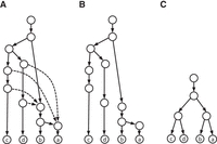
In this study, phylogenetic networks over a set of taxa are rooted, directed acyclic graphs in which leaves represent the taxa, the nonleaf indegree-1 nodes represent speciation events and the nodes with multiple incoming edges represent reticulation events. The nonleaf indegree-1 nodes are called tree nodes; the other nonleaf nodes are called reticulate nodes. We assume that each tree node is of outdegree 2; each reticulate node and the network root is of outdegree 1 in a phylogenetic network (Fig. 1). Phylogenetic trees are just phylogenetic networks with no reticulate nodes and thus are binary. (Basic concepts and notation can be found in the Supplemental Methods.)
The display of a phylogenetic tree in a tree–child network. (A) A tree–child network with two reticulate nodes on the taxa (a to d). (B) A subtree that was obtained by the removal of the dashed incoming edges of the reticulate nodes in the network. (C) A tree displayed in the network, which was obtained from the subtree in B by removing all degree-2 nodes through combining their unique incoming and outgoing edges into an edge.
Now that a variety of genomic projects have been completed, reticulate evolutionary events (e.g., horizontal gene transfer, introgression, and hybridization) have been shown to play important roles in genome evolution (Koonin et al. 2001; Gogarten and Townsend 2005; Marcussen et al. 2014; Fontaine et al. 2015). Although phylogenetic networks are appealing for modeling reticulate events (Koblmüller et al. 2007), it is extremely challenging to apply phylogenetic networks in the study of genome evolution. One reason for this is that a computer program has yet to be made available for analyzing data as large as what current research is interested in (Wu 2020; Molloy et al. 2021), although recently, Bayesian methods have been used to reconstruct reassortment networks, which describe patterns of ancestry in which lineages may have different parts of their genomes inherited from distinct parents (Müller et al. 2020, 2022).
Here, we focus on computing phylogenetic networks that display a given set of gene trees (Wu 2010; Albrecht et al. 2012; Whidden et al. 2013; Elworth et al. 2019; van Iersel et al. 2022). In this approach, trees are first inferred from biomolecular sequences and then used to reconstruct a phylogenetic network with the smallest hybridization number (HN) that displays all the trees (see Elworth et al. 2019), where the HN is defined as the sum over all the reticulate nodes of the indegree of each reticulate node minus 1. This approach takes advantage of the fact that the theory of phylogenetic trees is mature, and there are excellent tools available for inferring trees from a large number of sequences. It has been used in evolutionary studies (Koblmüller et al. 2007; Marcussen et al. 2014).
Although this parsimonious approach is faster than the maximum likelihood approach (Lutteropp et al. 2022), the parsimonious network inference problem is still NP-hard even for the special case when there are only two input trees (Bordewich and Semple 2007). For the two-tree case, the fastest programs include MCTS-CHN (Yamada et al. 2020) and HYBRIDIZATION NUMBER (Whidden et al. 2013). For the general case in which there are multiple input trees, HYBROSCALE (Albrecht 2015) and its predecessor (Albrecht et al. 2012), PRIN (Wu 2010), and PRINs (Mirzaei and Wu 2015) have been developed. All of these methods reconstruct a tree–child network with the smallest HN. Some of the methods insert reticulate edges or use other editing operations to search a network in the network space. Others reduce the tree–child network reconstruction problem to finding maximum acyclic agreement forests for the set input trees. Finally, some methods combine both of these techniques. Unfortunately, none of them will work for inferring a network from more than 30 trees if the trees have 30 or more taxa and do not have any nontrivial taxon clusters in common, where a nontrivial taxon cluster of a tree consists of all taxa below a tree node that is neither a leaf nor the root.
Because the network space is vast and cannot be fully sampled, attention has been switched to the inference of tree–child networks (Cardona et al. 2009), in which every nonleaf node has at least one child that is not reticulate, or, recently, a tree-based network (Pickrell and Pritchard 2012). Tree–child network is a superclass of phylogenetic trees with a completeness property that for any set of phylogenetic trees, there exists always a tree–child network that displays all the trees (Linz and Semple 2019). Other desired properties of tree–child networks include the fact that all the tree–child networks are efficiently enumerated (Zhang 2019a,b; Cardona and Zhang 2020).
Results
We mainly report a scalable computer program for inferring tree–child networks from multiple gene trees. The program ALTS takes a different approach that reduces the network inference problem to aligning the lineage taxon strings (LTSs) computed from the input trees with respect to (w.r.t.) an ordering on the taxa.
The inference algorithm
Consider a set X of taxa. Let T be a binary phylogenetic tree on X, and let N be a tree–child network on X. N displays T if T can be obtained from N by (1) removing all but one incoming edge for each reticulation node (Fig. 1A,B) and then (2) deleting all degree-2 nodes (which were reticulation nodes in N) (Fig. 1C).
The inference algorithm we introduce here will check all possible orderings on the taxon set to obtain the tree–child networks
with the smallest HN (and equivalently the smallest number of nodes). Let X be a taxon set such that |X| = n, and let π = π1π2 · · · πn, representing a (total) ordering of X, by which πi is “less than” πi+1 for each i < n. For any nonempty subset X′ of X, we use  and
and  to denote the minimum and maximum taxon of X′ w.r.t. π, respectively.
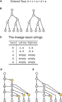
Because the root of T is of outdegree 1, T has n nonleaf nodes, called internal nodes. We label the n internal nodes of T one-to-one with the taxa w.r.t. π by assigning the smallest taxon to the degree-1 root and assigning  to an internal node with children v and w, where tv is the smallest taxon below v (Labeling) (Supplemental Methods). For instance, let X = {a, b, c, d, e} and π = bcade (Fig. 2A). The two trees on X in Figure 2B have their internal nodes labeled w.r.t. πusing Labeling.
The construction of a tree–child network that displays two phylogenetic trees. (A) An ordering on {a, b, c, d, e}. (B) Two trees, where the internal nodes are labeled w.r.t. the ordering using the Labeling algorithm. (C) The lineage taxon strings (LTSs) of the taxa obtained from the labeling in B. (D) The rooted directed graph constructed from the shortest common supersequences (SCS) of the LTSs of the taxa (in C) using Tree–child Network Reconstruction. The SCS is [c, e, a] for [c, a] and [c, e] and is [e, d, a] for [e, d] and [d, a]. (E) The tree–child network obtained after the removal of the degree-2 nodes.
Let τ be a specific taxon of X such that τ ≠ π1. We consider the unique path from the root ρ to the leaf ℓ that represents τ in T:  Then,
Then,  , whereas
  . Because
 , there is a unique index j such that 1 ≤ j < k and
  . This implies that uj was labeled with τ by applying Labeling and that no other internal node got the same label. The sequence consisting of the labels of
  is called the lineage taxon string (LTS) of τ. The LTSs computed in the trees given in Figure 2B are listed in Figure 2C.
Conversely, for the LTS of each taxon τ, we construct a directed path whose nodes are labeled one-to-one with the taxa of the LTS, and add a leaf labeled with τ below the path. After we connect the first node of the resulting path ending with each taxon other than π1 to all the nodes labeled with the taxon in other paths, we obtain T. Thus, the LTSs obtained from T under any ordering π on X can be used to recover uniquely T.
A string s is said to be a common supersequence of multiple strings if all the strings can be obtained from s by erasing zero or more symbols. Let  be a set of k trees on X. Let αji be the LTS of πi in Tj for each i from 1 to n. (Note that αjn is the empty string for each j.) Assume that, for each i, βi is a common supersequence of all
  on X. We can construct a tree–child network
  on X using the Tree–Child Network Construction algorithm given below.
1. (Vertical edges) For each βi, define a path Pi with |βi| + 2 nodes:

where βn is the empty sequence.
2. (Left–right edges) Arrange the n paths from left to right as  .
.
If the mth symbol of βi is πj, we add an edge (vim, hj) for each i and each m.
3. For each i > 1, if hi is of indegree 1, eliminate hi by removing hi, together with its incoming and outgoing edge, and adding a new edge from its parent to its child.
The algorithm is illustrated in Figure 2, D and E, where the SCSs are [c, e, a] and [e, d, a] for π1 = b and π2 = c, and the empty sequence for π3 = a and π4 = d.
The network output from Tree–Child Network Construction is always a tree–child network (Proposition 2) (Supplemental Methods). Combining Labeling and Tree–Child Network Construction, we obtain the following exact algorithm for the network inference problem, for which the correctness is proved in Section A of the Supplemental Methods.
Input: K trees  on X, |X| = n.
0. Set M = ∞ and define n − 1 string variables  ;
;
1. For each ordering π = π1π2 · · · πn on X:
1.1. Call Labeling to label the internal nodes in each Ti;
1.2. For each taxon πj, compute its LTS sij in each Ti;
1.3. Compute the SCS sj of  for each j < n;
1.4. If  , update M to the length sum; update Sj to sj for each j;
2. Call Tree–Child Network Construction to compute a tree–child network from the strings  .
.
A scalable version
Because there are n! possible orderings on n taxa and 15! is already too large, Algorithm A is not fast enough for a set of multiple trees on 15 or more taxa. Another obstacle to scalability is computing the SCS for the LTS of each taxon. We achieved high scalability by using an ordering sampling method and a progressive approach for the SCS problem.
First, the ordering sampling starts with an arbitrary ordering on the taxa and finishes in  iterative steps. Assume that Πm is the set of orderings obtained in the mth step (m ≥ 1) such that |Πm| ≤ H for a parameter H predefined to bound the running time. In the (m + 1) step, for each ordering π = π1π2 · · · πn ∈ Πm, we generate (n − 2m + 1)(n − 2m) new orderings by interchanging π2m−1 with πi and interchanging π2m with πj for every possible i and j such that i ≠ j, i > 2m and j > 2m. For each new ordering
  , we compute a SCS si of the LTSs of taxon
  in the input trees for each i ≤ 2m. We compute Πm+1 by sampling, at most, H new orderings that have the smallest length sum
  .
.
Second, different progressive approaches can be used to compute a short common supersequence for LTSs in each sampling step (Fraser 1995). We use the following approach:
-
A common supersequence of n strings is computed in n − 1 iterative steps. In each step, a pair of strings si and sj such that the SCS of si and sj, SCS(si, sj), has the minimum length, over all possible string pairs, is selected and replaced with SCS(si, sj).
Although the above algorithm had good performance for our purpose according to our test, it cannot always output the shortest solution for all possible instances. The reason is that finding the SCS for arbitrary strings is NP-hard in general (Garey and Johnson 1979), and our algorithm is as a linear-time algorithm unlikely to be the exact algorithm.
After the sampling process finishes, we obtain a set  of good ordering; for each ordering, we obtain a short common supersequence of the LTSs of a taxon obtained from the input
trees. To further improve the tree–child network solution, we also use the dynamic programming algorithm to recalculate a
short common supersequence for the LTSs of each taxon, subject to the 1 GB memory usage limit. We then use whichever is shorter
to compute a tree–child network.
Implementation of the algorithm
Another technique for improving the scalability is to decompose the input tree set into irreducible sets of trees if the input trees are reducible (Wu 2010; Albrecht et al. 2012) (Sec. B, Supplemental Methods). Here, a set of trees are reducible if there is at least one common cluster except the singletons and the whole taxon set.
Our program is named ALTS, an acronym for “Aligning Lineage Taxon Strings.” It can be downloaded from the GitHub site (see Software availability). We also developed a program that assigns a weight to each edge of the obtained tree–child network if the input trees are weighted (Sec. C, Supplemental Methods).
In summary, the process of reconstructing a parsimonious tree–child network involves the following steps. First, decompose
the input tree set S into irreducible tree sets, say  . Second, infer a set Ni of tree–child networks for each Si. Third, assemble the tree–child networks in
  to obtain the networks that display all the trees in S. Fourth, if the input trees are weighted, the branch weights are estimated for the output tree–child networks.
Validation experiments
We assessed the accuracy and scalability of ALTS on a collection of simulated data sets that were generated using an approach reported in Wu (2010) (see Methods section).
The optimality evaluation
We compared ALTS with two heuristic network inference programs: PRINs (Mirzaei and Wu 2015), which infers an arbitrary phylogenetic network, and van Iersel et al.’s method (van Iersel et al. 2022), which infers a tree–child network. We first ran the three methods on 50 sets of trees on 20 and 30 taxa, each containing 10 trees. Van Iersel et al.’s program is a parallel program. It could run successfully only on 44 (out of 50) tree sets in the 20-taxon case and 27 (out of 50) tree sets in the 30-taxon case. It was aborted for the remaining data sets after 24 h of clock time (or ∼1000 CPU hours) had elapsed.
ALTS outputs tree–child networks with the same HN as van Iersel et al.’s method on all but three data sets, where the latter ran successfully. The HN of the tree–child networks inferred with ALTS was one more than that inferred with the latter on two 20-taxon 10-tree data sets and three more than the latter on one 30-taxon 10-tree data set. Moreover, Van Iersel et al.’s method only outputted a tree–child network, whereas ALTS computed multiple tree–child networks with the same HN.
PRINs ran successfully on 49 out of 50 data sets in the 20-taxon case. In theory, the HN is inherently equal to or less than the HN of the optimal tree–child networks for every tree set. In the 20-taxon 10-tree case, the tree–child HN inferred with ALTS was equal to that inferred with PRINs on 20 data sets. The 29 discrepancy cases are summarized in the first row of Table 1. In the 30-taxon case, the HN difference of the two programs was also at most four (Table 1, row 2). The tree–child HN inferred by ALTS was even one less than the HN inferred by PRINs on one data set.
Summary of the HN discrepancy between ALTS and PRINs in 20-taxon and 30-taxon data sets each containing 10 trees
In summary, ALTS is almost as accurate as van Iersel et al.’s method in terms of minimizing network HN. The comparison between ALTS and PRINs indicated that the tree–child HN is rather close to the HN for multiple trees when the number of taxa is not too big.
The scalability evaluation
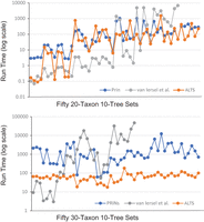
The wall-clock times of the three methods on 100 data sets, each having 10 trees on 20 or 30 taxa, are summarized in Figure 3. In the 20-taxa 10-tree case, the HN inferred by PRINs ranged from five to 17. ALTS finished in 0.09 sec to 25 min 14 sec (with the mean being 2 min 21 sec). On the 49 (out of 50) 20-taxa 10-tree data sets on which PRINs finished, it took 2.94 sec to 17 min 19 sec (with the mean being 2 min 58 sec). ALTS was faster than PRINs on 35 tree sets. On average, PRINs and ALTS were comparable in time for this case.
Run time (in seconds) of the three methods on 100 data sets. Each data set contains 10 trees on 20 or 30 taxa. The data sets are sorted in the increasing order according to the HN output from PRINs. Van Iersel et al.’s method had some missing data points because of an abort after 24 h of clock time.
On the 44 20-taxa 10-tree data sets on which van Iersel et al.’s method finished, its run time ranged from 0.07 sec to 82 min 22 sec (with the mean being 13 min 3 sec). Van Iersel et al.’s method ran faster than ALTS on 26 data sets in which the HN inferred by PRINs was less than 11. One reason for this is probably that the former is a parallel program. However, ALTS was faster than van Iersel et al.’s method on the remaining 18 tree sets in which the HN inferred by PRINs was 12 or more.
In the 30-taxon case, the HN of the solution from PRINs ranged from eight to 21. As shown in Figure 3, ALTS was faster than PRINs on every data set. Van Iersel et al.’s method finished on 31 (out of 50) data sets, for which the HN of the solution obtained with PRINs was 15 or more. ALTS was faster than Van Iersel et al.’s method on 23 data sets, whereas Van Iersel et al.’s method was faster than ALTS on the remaining eight data sets. On average, in the 30-taxon case, ALTS was 24 and 53 times faster than PRINs and the van Iersel et al.’s method, respectively.
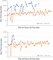
Lastly, we further ran ALTS on 100 data sets, each containing 50 trees on 40 or 50 taxa. PRINs finished on twenty-eight 40-taxon 50-tree data sets and five 50-taxon 50-tree data sets. In the 40-taxon 50-tree case, ALTS finished in 3 sec to 31 min 52 sec (with the mean being 7 min 14 sec). In contrast, PRINs finished on 28 tree sets, taking 3 min 19 sec to 15 h 34 min 52 sec (with the mean being 3 h 49 min 46 sec) (Fig. 4).
The run time (in seconds) of ALTS and PRINs on 100 data sets. Each data set contains 50 trees on 40 or 50 taxa. The data sets are sorted in the increasing order according to the HN of the tree–child networks inferred by ALTS. PRINs had some missing data points because of an abort after 24 h of clock time.
In the 50-taxon 50-tree case, ALTS finished in 2 sec to 45 min 12 sec (with the mean being 9 min 24 sec) (Fig. 4). In contrast, van Iersel et al's method could not finish on any irreducible set of 50 trees on 50 taxa. PRINs finished on five tree sets in 2 h 25 min on average (Fig. 4).
Taken together, these results suggest that ALTS has high scalability and is fast enough to infer tree–child networks for large tree sets.
The accuracy evaluation
Evaluating the accuracy of ALTS (and the other two methods) is not straightforward. The random networks that were used to generate the tree sets used in the last two subsections are not tree–child networks and contain frequently a large number of deep reticulation events. On the other hand, by the principle of parsimony, the networks inferred by the three programs contain far fewer numbers of reticulation events. As such, we assessed the accuracy of ALTS by using a Jaccard score that measures the symmetric difference between the set of clusters in the original networks and in the network inferred by ALTS (see Methods) (Huson et al. 2010).
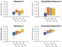
We considered two simulated networks containing 16 binary reticulations (Network 1) (Supplemental Fig. S1) and 19 binary reticulations (Network 2) (Supplemental Fig. S2). The two networks were produced using the same simulation program as used for the optimality evaluation but with a lower ratio of reticulation events. We also examined simplified versions of the two networks that were obtained by merging a reticulate node and its child if the reticulate node has a unique child and the child is also a reticulation node. The two simplified networks have nine and 10 reticulation events, respectively (Supplemental Figs. S1, S2, bottom). For each network and each k = 20, 30, 40, 50, we generated 10 k-tree sets. For each tree set, we inferred a network using ALTS and computed the Jaccard score for it and the original network. The dissimilarity analyses are summarized in Figure 5.
The box and whisker plots for the Jaccard scores for the original networks (Supplemental Figs. S1, S2) and ones inferred by ALTS in four cases. In each plot, the four bars from left to right summarize the Jaccard scores for the original network and 10 networks inferred from 20-, 30-, 40-, and 50-tree sets, respectively.
Network 1 (and its simplified version) contains fewer reticulation events than Network 2. We had slightly better reconstruction accuracy for Network 1 than Network 2 (mean Jaccard score range [0.3, 0.45] vs. [0.55, 0.65]) (Fig. 5). Also, the reconstruction from the trees sampled from each network was not significantly better than that from its simplified version. Given that all four networks can contain as many as 217 trees, the results suggest that 50 trees are far fewer than enough for accurate reconstruction of both nonbinary networks.
On the other hand, ALTS performed well for inferring a binary tree–child network with 13 binary reticulation nodes on 22 taxa. We sampled trees from the binary tree–child network given in Supplemental Figure S3. We could reconstruct the network on one out of 10 random five-tree sets, six out of 10 random 10-tree sets, and all 10 random 20-tree sets.
Last, we also examined the accuracy of reconstructing a network from the trees inferred from DNA sequence data using the following setting (for details, see Methods):
-
Generate randomly a network.
-
Sample a gene tree with branch lengths in the network.
-
Simulate DNA evolution to obtain a sequence of 1000 bp on the gene tree.
-
Infer a maximal likelihood tree from the simulated sequence.
On each random network, we sampled 2000 “true” gene trees and inferred 2000 trees accordingly.
We examined two networks (Network 3 and Network 4 hereafter) (Supplemental Fig. S4) on 30 taxa that contain five and six binary reticulation events, respectively. Because the inferred trees were noise, we used five-tree data sets for testing. Inference with more than five inferred trees had low accuracy, whereas inference with more than five true gene trees had high accuracy. We ran ALTS on 50 random tree sets for each of the three cases. In the first case, a data set consists of five inferred trees. In the second case, a data set consists of five “consensus” inferred trees that appeared six or more times in the list of inferred trees. Note that a consensus inferred tree is much more likely a true gene tree than a tree that was only inferred once in our experiment. In the third case, a data set consists of five “true” gene trees.
The results are summarized in Figure 6. For Network 3, the average Jaccard score for each inference test was 0.161, 0.079, and 0.043 in Case 1, 2, and 3, respectively. In addition, ALTS reconstructed Network 3 correctly on 27 out of 50 tree sets in Case 3. The performance of ALTS is similar for the testing on Network 4. These results suggest that accurate inference of gene trees from sequence data is vital for network inference with ALTS.
The box and whisker plots for the Jaccard scores for the original networks (Supplemental Fig. S4) and ones inferred using ALTS in three cases. In each plot, the three bars from left to right summarize the 50 Jaccard scores obtained using five random inferred trees (Case 1), using five random inferred trees that appeared six or more times in the list of all 2000 inferred trees (Case 2), and using the “true” gene trees (Case 3) sampled from the networks.
A phylogenetic network for 13 wheat-related grass species
We also validated our tool by inferring phylogenetic relationships for a set of wheat-related grass species. Bread wheat (Triticum aestivum) is a hexaploid species (genome AABBDD) formed through two rounds of hybridization between three diploid progenitors (i.e., Triticum urartu of the A subgenome, an unknown species of the B subgenome, and Aegilops tauschii of the D subgenome) (Marcussen et al. 2014; Levy and Feldman 2022). A recent comprehensive genomic study of Glémin et al. (2019) suggests that hybridizations were pervasive in the evolution of T. urartu, Se. tauschii, and 11 other grass species. Using a hypothesis testing approach, they detected six reliable and two possible reticulated events. Here, to eliminate the effect of incomplete lineage sorting (ILS) and tree inference errors, we simplified the 247 gene trees reported in their paper and selected 33 of them for network inference (see Methods section). Using ALTS, we obtained the phylogenetic network depicted in Figure 7. The network displays 73 out of 247 simplified gene trees and contains on average 79% nontrivial node clusters of the remaining trees.
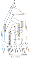
A phylogenetic network for 13 wheat-related grass species inferred using ALTS. The reticulation nodes are colored in yellow. The model contains two binary reticulate events (1 and 2) and four event clusters (3 to 6).
The network model contains two binary reticulate events and four clusters of reticulate events. Events 2 and 4 and event cluster 6 are consistent with the findings reported by Glémin et al. (2019). In particular, Event 2 is the hybridization between A and B lineages that formed the D-subgenome clade (Fig. 7, middle; Marcussen et al. 2014). The gene flows from an ancestor of Aegilops speltoides in the cluster 6 reveals that the Sitopsis species are closer to A. speltoides than to Ae. tauschii, consistent to the cytogenetic analyses reported by Kihara (1954). Our model also suggests that complex reticulate events (Cluster 5) occurred between Ae. tauschii and the ancestors of Aegilops caudata and Aegilops umbellulata. The complex gene flows in the event cluster 5 has not been reported in literature, but it is compatible with a chloroplast capture model (Fig. 2B; Li et al. 2015). Conversely, the two possible reticulate events reported by Glémin et al. (2019) are not supported by our model. Further verification of these inconsistent interspecific reticulate events may need gene order information on the related genomes and additional genomes of D-genome clade.
Discussion
We have presented ALTS. It is based on an algorithmic innovation that reduces the minimum tree–child network problem to computing the SCS of the LTSs of the taxa, obtained from the input trees w.r.t. a predefined ordering on the taxa. ALTS is fast enough to infer a parsimonious tree–child network for a set of 50 trees on 50 taxa in a quarter of an hour on average even if the input trees do not have any nontrivial taxon clusters in common. Another contribution is an algorithm for assigning weights to the edges of the reconstructed tree–child network if the input trees are weighted. Our work makes network reconstruction more feasible in the study of evolution and phylogenomics.
The accuracy analyses suggest that 50 trees are likely not enough for accurately inferring a phylogenetic network model that has 10 or more reticulation events. Therefore, a program that can process more than 100 trees is definitely wanted. We remark that ALTS can be made even more scalable by distributing the computing tasks for taxon orderings into a number of processors using distributed computing programming. This is because the computing tasks for different orderings are independent from each other.
Phylogenetic relationships obtained for the 13 wheat-related grass species and for Hominin (Sec. D, Supplemental Methods) provide an illustration of good performance of ALTS on empirical data. The analyses show that how to eliminate the effects of ILS is important for inference of phylogenetic networks. We will further investigate how to improve the accuracy of ALTS by incorporating the genomic sequences of the taxa and a process of removing ILS events into network inference.
Methods
Method for generating random tree data sets
The simulated tree data sets were generated using an approach appearing in work by Wu (2010). For each k ∈ {20, 30, 40, 50}, a phylogenetic network on k taxa was first generated by simulating speciation and reticulation events backward in time with the weight ratio of reticulation to speciation being set to 3:1. Fifty trees displayed in the networks were then randomly sampled. This process was repeated to generate 2500 trees for each k.
For assessing the accuracy of ALTS for inferring phylogenetic networks from genomic sequences, we generated gene trees with branch lengths from a network by calling a coalescent simulation program named ms (Hudson 2002). We ordered the speciation and reticulation events in the input network and set the time difference between adjacent evolutionary events to 10 coalescent units. Here, a relatively long coalescent time between adjacent evolutionary events was used to reduce the effect of ILS in the simulated gene trees.
Methods for gene sequence simulation and gene tree inference
We used the Seq-Gen program (Rimbaud and Grass 1997) with the GTR substitution model to generate DNA sequences of 1000 bp on a gene tree, where the scaling factor was set to 0.001 in order to convert coalescent units to the mutational units for Seq-Gen. Conversely, we used the RAxML program (Stamatakis 2014) with the GTR model to infer a gene tree from the simulated DNA sequence of 1000 bp. We used an outgroup to root the gene trees inferred by RAxML.
Jaccard score between two phylogenetic networks
We measured the dissimilarity between two phylogenetic networks by considering the symmetric difference of the set of taxa
clusters in the networks (Huson et al. 2010). Here, a cluster in a network consists of all taxa below a node in that network. Precisely, for two phylogenetic networks
N1 and N2 over X, we use C(Ni) to denote the multiset of clusters appearing in Ni for i = 1, 2, and define the Jaccard score between N1 and N2 as  .
.
Tree data preprocessing for wheat-related grass species
Two hundred forty-seven distinct gene trees for 13 wheat-related grass species and four outgroup species were downloaded from the evolutionary study of Glémin et al. (2019). (These trees were inferred from orthologous genes in 47 individual genomes by using RAxML v8.) To infer interspecific reticulate events, we simplified the gene trees by using only one individual sequence for each species and removing all four outgroup sequences, resulting in 227 distinct trees with 13 leaves. To reduce the effect of ILS and gene tree inferring errors, we further selected 33 gene trees for which either of the following two conditions is true: (1) it was inferred on two genes, and (2) every node cluster of it appears in t (=20) or more gene trees. We used the ratio of the number of trees displayed in a network to its HN to measure its expression capacity. The percentage used in the condition (2) was chosen to control the trade-off between the size and expression capacity of the network model. For t > 18, the inferred networks had a high HN. For t > 22, the inferred network displayed a low number of gene trees. For t = 18, 19, 20, 21, 22, the HN of the inferred network was 17, 13, 12, 12, and 12, whereas the network displayed 90, 71, 71, 71, and 63 gene trees, respectively. Because 90/17 < 71/13 < 71/12 and 63/12 < 71/12, we selected 20 as the filtering condition, resulting 33 gene trees.
Software availability
The C source code of ALTS can be found as Supplemental Code and at GitHub (https://github.com/LX-Zhang/AAST).
Competing interest statement
The authors declare no competing interests.
Acknowledgments
We thank Cedric Chauve and Aniket Mane for discussion in the beginning of this project. We also thank the anonymous reviewers for constructive comments on the earlier versions of our manuscript submitted to RECOMB'2023 and Genome Research. L.Z. was partly supported by Singapore Ministry of Education E Tier 1 grant R-146-000-318-114. Y.W. was partly supported by U.S. National Science Foundation grants CCF-1718093 and IIS-1909425.
Footnotes
-
[Supplemental material is available for this article.]
-
Article published online before print. Article, supplemental material, and publication date are at https://www.genome.org/cgi/doi/10.1101/gr.277669.123.
-
Freely available online through the Genome Research Open Access option.
- Received January 6, 2023.
- Accepted May 16, 2023.
This article, published in Genome Research, is available under a Creative Commons License (Attribution-NonCommercial 4.0 International), as described at http://creativecommons.org/licenses/by-nc/4.0/.


