

Abstract
Throughout evolution, genomes have acquired various repetitive elements, such as transposons, ribosomal DNA, duplicated genes, and tandem repeats. These sequences pose significant challenges to current high-throughput sequencing pipelines, which generate short reads that cannot be unambiguously mapped to reference genomes. We present an innovative algorithm, Hicberg, designed to leverage reads typically discarded by standard pipelines. Hicberg employs statistical inference coupled with probability distribution computation to accurately infer missing 3D contacts of repetitive elements within a genome from paired omic data, such as Hi-C data. Our results demonstrate that Hicberg provides new insights into the potential impact of repetitive elements on the spatial organization of genomes. Notably, we observed the positioning of molecular motors that create chromosomal loops associated with certain transposons in yeast. These findings underscore the importance of an integrative approach to better understand genomic complexity and pave the way for deeper explorations of repeated elements.
The spatial organization of chromosomes or whole genomes involves different levels of structure, such as chromosomal domains or loops, which can be linked to the cell's biological functions. In parallel with superresolution microscopy technologies, chromosome conformation capture (3C) approaches coupled with high-throughput sequencing (Hi-C) have been developed to explore the spatial organization of a genome at different scales (Dekker et al. 2002; Lieberman-Aiden et al. 2009). These technologies are based on the capture of DNA fragments that are in physical contact by fixation with a cross-linking agent combined with high-throughput sequencing to obtain the contact frequencies of different loci within a genome through the formation of chimeric DNA molecules (Lieberman-Aiden et al. 2009). Such methods allow the quantification of contacts between different loci computed on a population of cells and reveal a wide range of three-dimensional chromatin structures that can be involved in various biological processes, such as DNA replication and segregation (Dekker and Mirny 2024), gene regulation (Yang and Hansen 2024), or cell differentiation (Karpinska et al. 2025). Unusual genome organization can also be observed in disrupted biological functions such as cancer in humans (Wang et al. 2022) or infection (Wei and Ho 2022).
To address the growing amount of Hi-C data produced by the community, numerous analysis tools and pipelines have been proposed covering a variety of functions, notably to process, filter, and normalize (Forcato et al. 2017); detect loops (Fang et al. 2022) and topological domains (Fang et al. 2022); and quantify compartment signals (Chakraborty et al. 2022).
Many so-called up-scaling methods are also currently being developed to increase the resolution of Hi-C data that are, for example, sparsely covered. In particular, many of these methods use training phases to transform low-coverage data into high-coverage data, thereby enabling higher resolutions (Zhang et al. 2018; Carron et al. 2019; Hu and Ma 2021). However, these methods do not handle regions containing repetitive sequences that have multiple ambiguous alignments and leave these regions without a signal.
Indeed, as with other types of high-throughput sequencing and associated downstream analysis pipelines, the size of the generated reads, which is limited, for example, to the order of 50 bp, can lead to ambiguous mapping within the genome during the alignment process. Consequently, Hi-C analysis pipelines are limited to the exploitation of read pairs in which both partners of the pair align to unique genomic positions (uniquely mapping reads). Read pairs in which one partner of both partners can be mapped at several positions (multimapping reads) are traditionally filtered out, leading to a significant loss of information on the spatial organization of the genome, representing ∼15% of the standard Hi-C library for yeast and up to 35% of the Hi-C libraries for humans (Supplemental Fig. S1). These portions of the genome with repeated sequences remain invisible, appearing as empty bins, namely, white lines and columns on Hi-C contact maps.
However, various analyses have shown that repeated elements could play a fundamental role in metazoan genome folding (Cournac et al. 2016), in the genome organization of filamentous fungi (Winter et al. 2018), in the immune escape of apicomplexan parasites such as Plasmodium falciparum (Bunnik et al. 2018), or in the superintegron structure in Vibrio cholerae (Marin and Vicente 2013). One interesting recent example is the case of primate-specific endogenous retrotransposon human endogenous retrovirus subfamily H (HERV-H), which has recently been highlighted in the formation of topologically associating domains (TADs) (Zhang et al. 2019). Hence, characterizing the role of repeated elements in the three-dimensional structure of genomes remains a challenge that needs to be investigated.
To our knowledge, very few pipelines have been proposed to offer a reasonable solution for processing reads with ambiguous alignments in Hi-C or Micro-C experiments, and to date, there is only one pipeline addressing this issue called mHi-C (Zheng et al. 2019), which reallocates some of the ambiguous reads using some paired-end Hi-C read features. This pipeline allows fractional contact (i.e., multiple genomic coordinates can be assigned for one given Hi-C read pair), which can make signals difficult to interpret. This proposed answer remains partial, leaving out a significant proportion of reads that are not reallocated.
Here, we propose Hicberg, a computational approach that enables Hi-C data processing and maximizes the rescue of multimapping reads through a statistical inference based on the computation of statistical trends derived from both polymer physics and the technical features of Hi-C protocols. This approach paves the way for a deeper characterization and understanding of repeated elements in the context of the spatial organization of genomes. Although initially developed for processing data from 3C-derived capture techniques, Hicberg can also be used to process other paired-end omics, such as MNase-seq or ChIP-seq. This allows contact signals and other genomic signals to be confronted in the same computational framework, allowing a more exhaustive exploration of signals from repeated elements.
Results
The algorithm's operating principle of Hicberg
The operating principle of the computational method we propose here is to compute and use statistical trends present in the uniquely mapping part of the data to determine the probability of the different genomic positions of possible alignments of multimapping reads (Fig. 1).
General principles of the Hicberg method for the reconstruction of contact maps and genomic tracks. Read pair reconstruction involves classification into three groups (nonmapping, uniquely mapping, and multimapping reads). The uniquely mapping fraction of reads is used to profile the statistical trends of the data. Several components can be included in the statistical model: chromatin polymeric behavior P(s), genome coverage, and others. The statistical model computes the propensities for each potential contact to occur, and the propensity distribution is built. For each ambiguous pair, a single possibility is then chosen according to the propensity distribution.
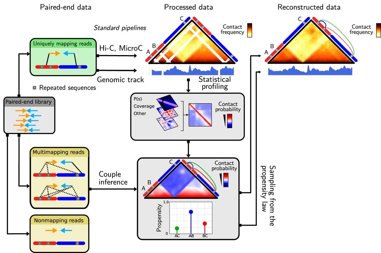
Hicberg used paired-end high-throughput sequencing data such as the Hi-C library and a reference genome as inputs. Each of the two mates is independently aligned to the reference genome via mapper software such as Bowtie 2 (Langmead and Salzberg 2012). The alignment procedure is performed so that all possible alignment positions for an ambiguous read are given. In the case of complex genomes rich in repeated elements, a partial report of the different alignment possibilities for an ambiguous read (e.g., 100 possible alignments) can be used to limit the use of computational resources.
Hicberg then classified pairs of reads into three different groups (Fig. 1; Supplemental Fig. S1B): nonmapping pairs, uniquely mapping pairs, and multimapping pairs. Nonmapping pairs have at least one read that does not align to the reference genome (which could be because of contamination, errors from sequencing, the presence of adapters, chimeric reads, etc.) and are excluded. Uniquely mapping pairs are those in which both reads uniquely align on the reference genome. These pairs are retained and used to build the statistical model. Multimapping pairs have at least one mate with more than one possible alignment; namely, the alignment quality is below a user-defined quality threshold (by default, mapq > 35). The pairs of reads belonging to this last group are those that are reassigned via the statistical model.
Statistical trends are computed via the fraction of uniquely mapping read pairs. The statistical model can rely on several tendencies present in the data. First, chromosomes can be characterized by their polymer behavior (Rippe 2001). Constrained by thermodynamics, in the case of intrachromosomal contacts, two loci are more likely to interact at short distances than at long distances. This observation is known as the distance law or P(s), which represents the probability (or normalized frequency) that two loci separated by distance s are in contact (Dekker et al. 2013). The distance law can be split into three different sublaws, taking into account the directionalities of the aligned reads and reflecting the different possible read configurations associated with the Hi-C protocol (Methods) (Supplemental Fig. S1C; Cournac et al. 2012; Matthey-Doret et al. 2022). Calculating contact frequency laws based on genomic distances while taking into account the directionality of the reads is essential for accounting for all the events that make up a Hi-C library. Indeed, many noninformative events such as undigested fragments and recircularization events (Supplemental Fig. S1C) can constitute a significant portion of the data. We chose to reconstruct this type of event as well to obtain data that most accurately reflects the reality of the experience. This is a key difference in the mHi-C method, which includes several upstream event filters prior to reconstruction.
Second, genome coverage (number of reads at each bin along the genome) is not necessarily uniform (Supplemental Fig. S1A). Therefore, the greater the coverage of a genomic region is, the greater the probability that a read will come from that region. This statistical trend can be discriminating when it presents a particular profile, such as for bacteria undergoing rapid growth, in which the region close to the origin of replication is naturally two to four times more covered than the region close to the replication terminus (Supplemental Fig. S1A). Such variation in genomic coverage can thus be used as a selective component for the relocation of multimapping pairs.
Each of the descriptors outlined above are evaluated and combined. In this way, each plausible pair of reads is assigned a propensity, forming a discrete probability distribution for all possible pairs. One pair of reads is then chosen by a random draw according to this probability distribution. Ambiguous read pairs whose genomic coordinates have been inferred are then aggregated with uniquely mapping pairs, enabling the establishment of complete genomic data sets.
Benchmark of Hicberg
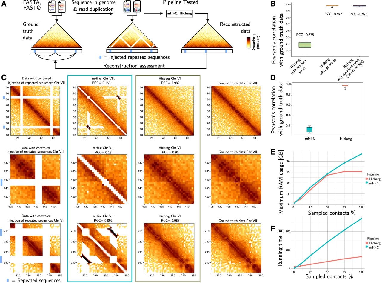
We first assessed the quality of the reconstructions proposed by Hicberg via data-driven simulations based on in silico modification of reference genome and Hi-C input files (Methods) (Fig. 2A). The benchmark strategy is based on a controlled injection of repeated sequences for certain regions. The reference genome is changed to have a sequence duplicated in the FASTA file, and all reads corresponding to the chosen repeated sequences are converted to generate alternative input FASTQ files of the paired-end data on which Hicberg is applied. The genomic data are reconstructed and compared with the ground truth via Pearson's correlation.
In silico bench testing strategy for assessing the quality of Hicberg reconstructions. (A) Controlled ambiguity is injected by duplicating sequences and selected reads in the FASTA and FASTQ files at chosen positions. This ambiguity is then confronted with Hicberg reconstruction after profiling and statistical inference. The ground truth and the data reconstructed through Hicberg are compared to assess the quality of the proposed reconstruction via the Pearson's correlation coefficient (PCC). (B) Comparison of the Hicberg method with three different modes of determination of contact probabilities: random mode (uniform distribution between the different contacts) and P(s) mode using the frequency of contact in function of genomic distance, with standard mode using in addition the genomic coverage. (C) Comparison of the mHi-C and Hicberg methods evaluated using the benchmark shown for three different representative regions: from left to right; contact map from data with controlled injection of repeated elements (blue boxes), with data reconstructed with mHi-C, with data reconstructed with Hicberg, and from ground-truth data. PCCs with the ground-truth data are given for mHi-C and Hicberg reconstructions. (D) Comparison of the mHi-C and Hicberg methods evaluated using the benchmark. The box plot shows the distribution of 24 comparisons using the PCC between the reconstructed region and the same region derived from the ground-truth data. (E) Memory usage of both Hicberg and mHi-C according to the subsampling of Hi-C data of S. cerevisiae from 5% to 100% of the 47 million pairs of reads of the data. (F) Runtime of both Hicberg and mHi-C according to the subsampling of Hi-C data of S. cerevisiae from 5% to 100% of the 47 million pairs of reads in the data.
We include a “random” mode, in which equal probabilities are assigned to all possible alignments (more specifically, if there are N possible alignments, it assigns a probability of 1/N to each one). This mode is used to illustrate how reconstructed signals behave when no specific statistical trend is used in the computation of probabilities.
We first tested the Hicberg method with three different modes of determination of contact probabilities: “random mode” (uniform distribution between the different contacts), “P(s) mode” using the frequency of contact in function of genomic distance, and “standard mode” using in addition the genomic coverage (Fig. 2B). It can be seen that the statistical trend of the P(s) distributions is the key factor in distinguishing and faithfully reconstructing the ground-truth data. The addition of genomic coverage has almost no impact.
Given the exhaustive nature of the scenarios that could be tested, we have chosen to limit ourselves to evaluations close to biological scenarios. The first parameter that can be tested concerns the number of repeated sequences within a genome. Hicberg shows strong stability to the number of repeated sequences, with a reconstruction score above 0.9 for a number of 50 when used in the standard mode (which takes into account P(s) and genomic coverage) in Saccharomyces cerevisiae. The correlation coefficient decreases sharply when the random mode is used reaching approximately 0.12 under these conditions (Supplemental Fig. S2C).
We also measured the quality of the reconstructions proposed by Hicberg as a function of the distance separating two repeated elements in S. cerevisiae. We observed relative stability, with reconstruction quality scores above 0.9 for separations between repeated sequences increasing from 5 to 200 kb in standard mode, whereas scores between 0.55 and 0.75 on average were obtained for the same separations in random mode (Supplemental Fig. S2C). The dispersion of the reconstruction quality scores is also greater when a random model is used. Finally, we evaluated the quality of the reconstructions according to the size of the repeated sequences. Hicberg shows robustness with respect to this parameter, with reconstruction qualities more than 0.97 up to 20 kb in S. cerevisiae in standard mode, compared with scores of less than 0.6 with a random model (Supplemental Fig. S2C).
The reconstructions are similar even if the seed for the random seed is changed (Supplemental Fig. S2B). Importantly, selecting from a probability distribution is a crucial step in allowing the statistical inference engine to explore and select events that can be rare but present in the data set. In fact, systematically selecting the contact with the highest probability would mean that certain contacts would go undetected, which would create imbalances in the reconstructions and produce aberrant signals (Supplemental Fig. S2B).
We then compare the mHi-C and Hicberg methods evaluated using our benchmark. To illustrate the constructions of the two methods, we show three different representative regions from data with controlled injection of repeated elements, from data reconstructed with mHi-C, from data reconstructed with Hicberg, and from ground-truth data (Fig. 2C).
The distribution of 24 comparisons using Pearson's correlation coefficient (PCC) between the reconstructed region and the same region derived from the ground-truth data shows that the Hicberg approach is much closer to the ground-truth data compared with the mHi-C approach in our test bench (Fig. 2D).
For comparison with computer resources, we ran Hicberg and mHi-C on standard Hi-C data from an asynchronous S. cerevisiae yeast population (Methods) with a sequencing depth of 47 million reads. Hicberg outperforms mHi-C in terms of both RAM usage and computing time. The Hicberg RAM consumption level remains well below mHi-C regardless of the level of data subsampling (Fig. 2E). In terms of computation time, when 16 CPUs are used, contact map reconstruction with 2 kb resolution according to standard parameters is achieved in 63 min with Hicberg versus 270 min for mHi-C from read alignment to contact map construction without library subsampling (Fig. 2F).
A major difference between Hicberg and mHi-C is the tolerance of contact splitting for a pair of reads to be reassigned (i.e., the possibility of assigning several genomic coordinates to a given pair of reads). Our choice with Hicberg not to tolerate this splitting makes absolute comparison of genomic track reconstructions via our strategy complex. Indeed, using the standard mHi-C parameters, we obtain matrices with a greater overall number of contacts than the number of initial reads in the library under study. Although not quantitatively evaluable according to the modality set for the Hicberg benchmark, the quality of the reconstructions proposed by our method and mHi-C can be visually appreciated. Indeed, the reconstructions proposed by mHi-C of the subtelomeric regions of Chromosomes IX and X in S. cerevisiae (Supplemental Fig. S3A,B) show an absence of contact reattribution and therefore an absence of correctly defined structuring of these regions in contrast to the structuring proposed by Hicberg. A similar observation can be made for reconstructions of the peripheral region of ribosomal DNA (rDNA) located on Chromosome XII in S. cerevisiae. This region, previously absent from contact maps, is very poorly reconstructed via mHi-C, whereas a clearly defined structure, showing local chromatin compaction, was revealed by Hicberg (Supplemental Fig. S3C). Finally, some specific regions, such as those located on Chromosomes VII and XIV, presented medium-range artifactual patterns after mHi-C reconstruction, even though these patterns were absent from Hicberg reconstructions (Supplemental Fig. S3D,E).
Reconstruction of real genomic data in S. cerevisiae
To illustrate examples of new biological analyses that can be performed via Hicberg reconstructions, we first focus on reconstructions of chromosome contact maps in the model organism S. cerevisiae. This yeast has a medium-sized genome of 12.5 Mb, with diverse sources of repeated sequences: It has five long terminal repeat (LTR)–retrotransposon families called Ty1, Ty2, Ty3, Ty4, and Ty5 (Bonnet and Lesage 2021), with approximately 50 elements distributed across all chromosomes. It contains the rDNA region, which consists of a 100- to 150-copy locus repeat. It also contains repeated sequences in telomeric regions, which mainly contain two types of repeated elements, called “X” and “Y.” Finally, it contains several duplicated genes (e.g., CUP1 on Chromosome VIII). For alignment, we used the genome sequences recently obtained for the telomere-to-telomere (T2T) quality (O'Donnell et al. 2023; Miao et al. 2025) associated with the online database ScRAPdb (see Methods).
We started performing Hicberg reconstructions on an example of standard Hi-C libraries (using a commercial kit; Methods) for the yeast S. cerevisiae under normal growth conditions and for an asynchronous population. Without Hicberg reconstruction and with standard filtering of ambiguous reads, 35.3 million exploitable reads remained over the initial 47 million. With Hicberg reconstruction, there are 42.3 million exploitable reads, representing 7 million additional pairs of reads, that is, an information gain of 20%. The remaining 5 million read pairs had at least one of the two reads that was chimeric or nonmapping owing to sequencing errors or mutations, sequencer noise, etc.
If we calculate in terms of usable bins, for a standard Hi-C library of S. cerevisiae yeast, 8.2% of bins are under-covered (the threshold is five median absolute deviations below the median log marginal sum). After Hicberg reconstruction, the percentage of bins with low read counts that cannot be used drops to 0.6% (Fig. 3A). These bins correspond in particular to regions of the genome that are poor in restriction sites used in the Hi-C protocol (examples are given in the following section).
Examples of Hicberg reconstructions in the genome of the model organism S. cerevisiae. (A) Distribution of the number of reads per bin for standard Hi-C experiment in yeast S. cerevisiae without and with Hicberg reconstruction. The threshold used to filter bins with few reads before normalization corresponds to five median absolute deviations below the median log marginal sum and is represented by a dashed line. (B) Chromosome contact map without and with Hicberg reconstruction for Chromosome VII (bin = 2 kb, with normalization) (C) Mappability signal along the Chromosome VII. (D) Hi-C coverage before (green) and after (blue) Hicberg reconstruction. (E) Examples of reconstructions at representative regions: on several yeast transposons (Ty) at Chr VII, between both telomeres TEL-L and TEL-R of Chr VII, between centromeres of Chr VII and Chr X, and between telomeres TEL-L of Chr VII and TEL-L of Chr X with Hi-C coverages without and with reconstruction. (F) Detection of chromosomal loops and borders on data without and with reconstruction. Pileup plots for detected loops and borders for both types of data are shown as well as average signal around anchors of ChIP-seq signal of Scc1, a cohesin subunit.
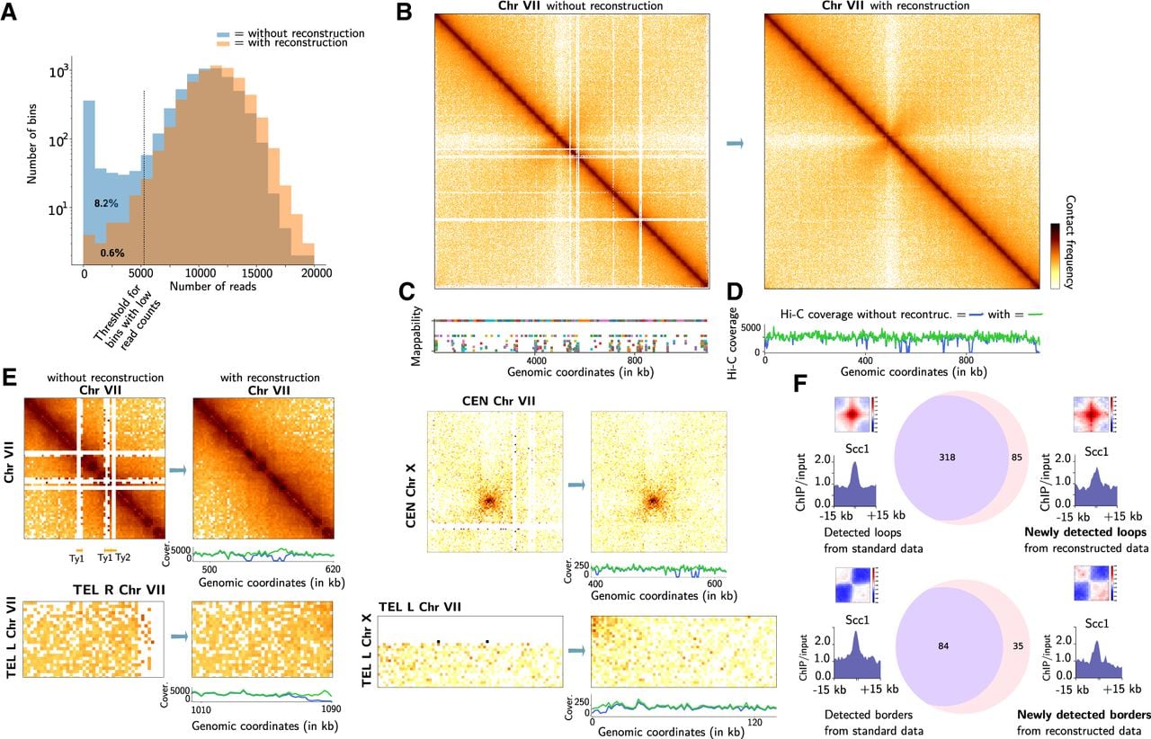
We present examples of Chromosome VII reconstruction (Fig. 3B–D) and of all chromosomes (Supplemental Fig. S4–S21). The coverage of the reconstructed parts reaches a normal level for the whole chromosome, and the contact map shows a homogeneous signal on all the different chromosomes. With respect to reconstruction, some regions still have very low coverage. This is the case for Chromosome I, for example, in which several bins show low Hi-C coverage with reconstruction (Supplemental Fig. S4). Gene annotation revealed that these genes correspond in particular to those of the FLO family (e.g., FLO9 and FLO1 for the Chromosome I). Computation of the number of restriction sites used in the Hi-C protocol (DpnII, HinfI) revealed that all FLO genes were deficient in these restriction sites (with the exception of the FLO8 gene on Chromosome V) (Supplemental Fig. S21). On the basis of the Hi-C data from a similar type of protocol, it was proposed (Ruault et al. 2021; Lazar-Stefanita et al. 2022) that these genes present contact enrichment. The fact that these genes are restriction site deficient has a significant impact on their detectability, and different protocols are needed to study contacts between FLO genes. This highlights the fact that Hicberg can uncover regions that are difficult to detect apart from mapping problems.
Hicberg reconstructs specific contact signals between telomeres on the same chromosome or between different chromosomes (Fig. 3E). These signals are important biologically, as they depend on the cell state and metabolism. For example, in quiescent cells, the grouping of telomeres into a unique focus or hypercluster localized in the center of the nucleus has been shown (Guidi et al. 2015; Ruault et al. 2021).
Chromosome reconstructions revealed interesting contact patterns, such as the presence of chromosomal domains at subtelomeric regions such as Chromosome IX (Supplemental Fig. S11B) or Chromosome XIII (Supplemental Fig. S15B). We also observed a border pattern at the Hidden MAT Left (HML) locus on Chromosome III (Supplemental Fig. S6B), which recalls the border pattern at the Hidden MAT Right (HMR) locus visible in the data without reconstruction (Supplemental Fig. S6B). Interestingly, these loci have been recently proposed to be associated with loop extrusion processes with condensin complexes (Piveteau et al. 2026).
We also present two examples of contact maps between two different chromosomes (Supplemental Fig. S20). Reconstructions can show lines in depleted areas of contact (notably at centromeres). However, these reads represent a very small proportion of the signal.
Finally, we generated a mitochondrial contact map (Supplemental Fig. S19). Although reconstruction with Hicberg only slightly increases map coverage, it is possible to see an interaction domain at the level of the large COX1 gene (size, 12.8 kb), reminiscent of domain structures observed in bacterial genomes (Bignaud et al. 2024).
To determine the biological relevance of the data reconstructed by Hicberg, we detected typical chromosome loop and domain boundaries patterns in Hi-C data with and without reconstruction (Fig. 3F). We used Hi-C data from S. cerevisiae synchronized in the G2/M phase of the mitotic cell cycle (Supplemental Table S1). During this phase, it is now well established that cohesin loops form along S. cerevisiae chromosomes to ensure genome-wide condensation (Costantino et al. 2020; Dauban et al. 2020). The majority of the loops detected therefore show cohesin enrichment at their anchors in the data without reconstruction. This is visible in the average ChIP-seq signal profile of Scc1 at the loop anchor positions, Scc1 is a subunit of cohesin. Interestingly, using the reconstructed data, a greater number of loops are detected (corresponding to a 27% increase). Cohesin enrichment is also visible on the newly detected loops, showing that the detections on the reconstructed data are consistent with the expected biology. A similar analysis is performed with the detection of domain boundaries, in which the use of data reconstructed by Hicberg represents a 41% increase in the number of boundaries detected, with the signature of cohesin enrichment also present in the newly identified boundaries. Examples of newly detected chromosomal loops and associated repeated sequences will be described in the following sections.
Hicberg can detect changes in repeated sequence positions in a reference genome
Aberrant contact patterns can appear in several contact maps, for example, at Chromosome III and Chromosome XII, with reconstructions using the current reference genome of the Saccharomyces Genome Database (SGD) (genome assembly R64, GCF_000146045.2, sacCer3) instead of the T2T assembly (Supplemental Fig. S22A). By plotting the 4C-like contact signal as, for example, from a family of Ty1 retrotransposons (Methods), it is possible to detect peaks at regions that are not annotated as carrying a Ty (Supplemental Fig. S22B,C). Indeed, this type of approach allowed the identification of the presence of a Ty1 on Chromosome XII that is not annotated in the sacCer3 version of the S. cerevisiae S288C genome. A PCR experiment followed by Sanger sequencing confirmed the presence of Ty1 at this genomic position (Methods) (Supplemental Fig. S22D). This finding shows that Hicberg can also reveal the presence of repetitive sequences that might be omitted from the reference genome. Although it is not intended to replace a long-read approach (Oxford Nanopore Technologies [ONT], Pacific Biosciences [PacBio]) for genome-wide annotation of repetitive sequences, it can locally detect the presence of one or more repetitive sequences absent from a reference genome.
Reconstruction of genomic data in bacteria
Finally, we present two examples from the bacterial world: The first example corresponds to the reconstruction of a contact map of the genome of the bacterium Escherichia coli (Cockram et al. 2021), which contains a duplicated region of several kilobases (Supplemental Fig. S23). The reconstruction shows a map consistent with the layout of the duplication, enabling us to check the geometry and correct positioning of genetic constructs within the genome involving repetitions. We also present an example of a reconstruction for the V. cholerae bacterium, which contains two chromosomes (Supplemental Fig. S24). The reconstruction is able to produce a contact pattern between the two chromosomes, notably at the level of the superintegron on Chromosome 2, which harbors hundreds of gene cassettes (Rowe-Magnus et al. 1999).
Hicberg is able to reconstruct signals linked to compartmental organization
To explore the potential of Hicberg reconstructions with complex contact signals, we reconstructed several Hi-C data sets of organisms that have compartment signals. This characteristic of the spatial organization of genomes, particularly in eukaryotes, notably in humans (Lieberman-Aiden et al. 2009), corresponds to a bipartitioning of the genome into two compartments: One, known as compartment A, is rather active at the transcriptional level and contains genes; the another, known as compartment B, is rather silent and contains fewer genes. This signal is particularly visible on the correlation matrix in the form of a checkered pattern (Chakraborty et al. 2022). Our laboratory has recently artificially created a compartment signal in chimeric S. cerevisiae strains that contain pieces of the Mycoplasma mycoides bacterial chromosome on Chromosome XVI (Meneu et al. 2025). This chromosome alternates between a yeast chromosome with a GC content of ∼38% and an M. mycoides chromosome with a GC content of ∼20% (Fig. 4A).
Compartment reconstruction signals by Hicberg. (A) Normalized contact map of the chimeric Chromosome XVI of S. cerevisiae and M. mycoides binned at 5 kb resolution without and with Hicberg reconstruction. The GC content of the sequences and annotations for S. cerevisiae and M. mycoides are shown below the left panel, and the Hi-C coverages before (blue) and after (green) the Hicberg reconstructions are shown below the right panel. (B) Correlation matrices of the chimeric Chromosome XVI of S. cerevisiae and M. mycoides binned at 5 kb resolution without and with reconstruction. The GC content is shown below the map on the right. (C) Normalized contact map of Chromosome 5 of Epichloë festucae binned at 10 kb resolution without and with reconstruction. Hi-C coverages before (blue) and after (green) Hicberg reconstruction are shown below the right panel. (D) Correlation matrices of Chromosome 5 of E. festucae binned at 10 kb resolution without and with reconstruction. The GC content (orange) is shown below the map on the right. A zoom-in of the contact map is shown in relation to the GC content signal below.
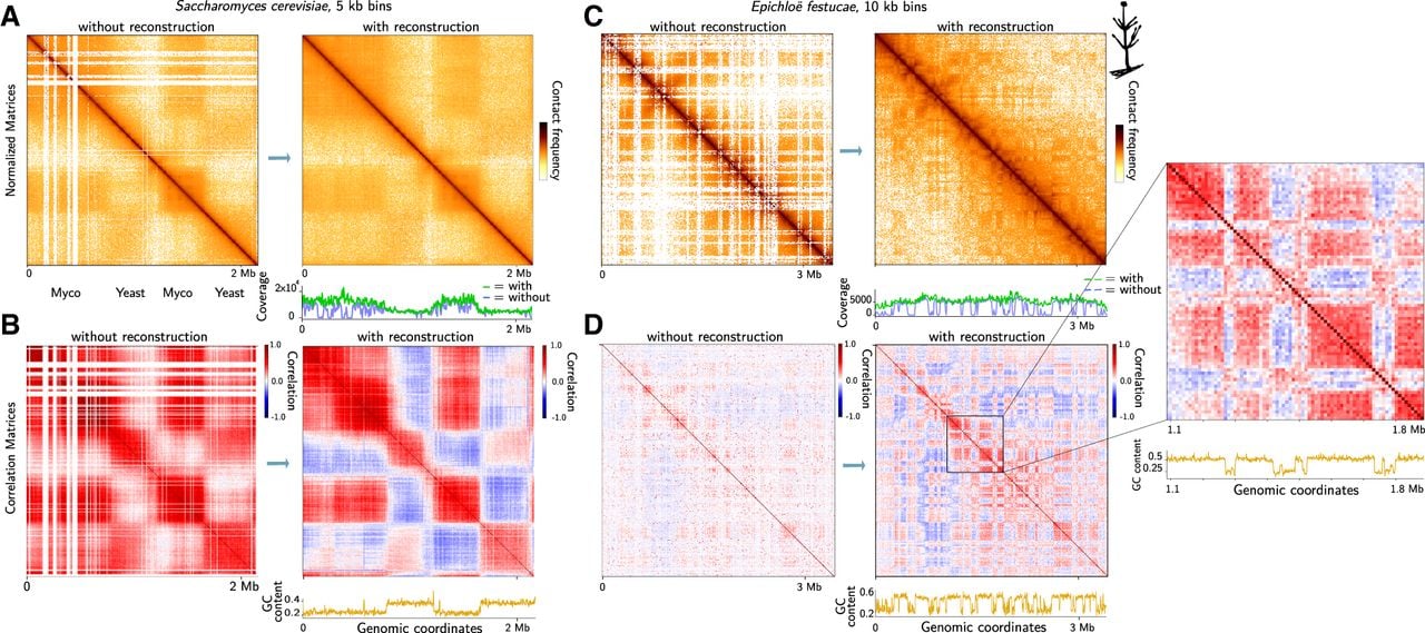
M. mycoides bacteria contain several repeated sequences, particularly insertion sequences (ISs), which are bacterial transposons that can affect genome organization and plasticity (Thiaucourt et al. 2011). These regions generate white lines at the IS regions in the contact maps processed with standard pipelines. With the Hicberg reconstructions, the normalized contact map shows a homogeneous signal over the whole chromosome, including the repeated sequences present on the M. mycoides segments (Fig. 4A). Interestingly, if we plot the 4C signal, such as that of the telomeric region present only in the reconstructed data, we can observe that the signal shows nonmonotonic behavior with increases in intermediary genomic distances in the contact signal following the organization of the compartments (Supplemental Fig. S25).
The computation of the correlation matrix used to highlight the compartment signals is much clearer, with a stronger correlation signal across the whole matrix (Fig. 4B). Although the Hicberg reconstructions on the normalized matrices mainly modify the lines with poor coverage, the effect of the Hicberg reconstructions on the correlation matrices, which calculate for each pixel the correlation coefficient between the whole row and the whole column, influences the whole correlation matrix (Fig. 4B).
We then tested it on other microorganisms naturally containing a high proportion of repeated sequences. For example, we tested it on the organism Epichloë festucae, which is a filamentous fungus known to have a high proportion of repeated sequences in its genome, notably LTR retrotransposons, miniature inverted repeat transposable elements (MITEs) (Fleetwood et al. 2011), and DNA transposons. It was shown that repeated elements play a key role in the nuclear organization of E. festucae. These repeated elements help to divide the genome into distinct regions with similar gene expression profiles (Winter et al. 2018). Without reconstruction, a large proportion of reads are below the mapping threshold of standard pipelines, generating many empty lines or presenting an unusable weak contact signal (Fig. 4C). The Hi-C coverage signal shows a very inhomogeneous profile with many undetectable regions. The correlation matrix used to highlight the compartment signals is also poor in exploitable signals, and only a restricted part of the genome allows us to observe a checkerboard signal typical of the behavior of the signal in the compartments (Fig. 4D). With Hicberg reconstruction, the contact map is filled with signals, the Hi-C coverage becomes homogeneous, and the compartment signal can now be observed at the scale of the chromosome and the whole genome. Interestingly, this confirms the link with GC content: Genomic regions with similar GC contents are present in the same compartment (Fig. 4D, zoom).
Both of these examples of reconstructions display Hicberg's ability to reconstruct signals that deviate from the average behavior mediated by contact frequency as a function of genomic distance, P(s). Indeed, the reads present in the data set that are generally excluded for analysis provide sufficient constraints for signal prediction and allow the reconstruction of more complex signals for compartment signals.
The 2µ parasitic plasmid shows enriched contact with Ty transposons
The 2µ plasmid is a natural plasmid present in the nucleus of laboratory or natural strains of S. cerevisiae (McQuaid et al. 2019). It is 6.4 kb in size and does not appear to confer any advantage on its host (Chan et al. 2013). It has very high stability, close to that of its host chromosomes, potentially because of a hitchhiking mechanism (Sau et al. 2019). Recently, the 2µ plasmid was shown to preferentially contact long regions with low transcriptional activity (Girard et al. 2025). Compared with the average size of genes (1.5 kb) of the host organism, Ty retrotransposons in the yeast S. cerevisiae are also rather large (Curcio et al. 2015), with a size of ∼5.5 kb. The transcription of these genes is generally low compared with that of the rest of the genome (Morillon et al. 2002). They meet the two criteria that make them potential hot spots of contact for the 2µ plasmid. To test this hypothesis, we reconstructed the contact signals of the 2µ plasmid with the different elements making up the Ty1, Ty2, and Ty4 families. The contact signal of the 2µ plasmid is enriched with various Ty elements (Fig. 5A–D).
Parasitic 2µ plasmid shows contact enrichment with yeast transposons. (A) Contact map of Chromosome VI of S. cerevisiae without reconstruction; bin = 2 kb in the asynchronous population (BY4741 strain). Below is the contact signal of the 2µ plasmid along Chromosome VI without reconstruction. (B) Heatmap representing the contact signals of the 2µ plasmid with three different families of yeast transposons: Ty1 (31 elements), Ty2 (13 elements), and Ty4 (3 elements) without reconstruction. Below is the averaged signal (in blue) over the different elements of each family. (C) Contact map of Chromosome VI of S. cerevisiae with reconstruction, bin = 2 kb. Below is the contact signal of the 2µ plasmid along Chromosome VI with reconstruction. (D) Heatmap representing the contact signals of the 2µ plasmid with three different families of yeast transposons: Ty1, Ty2, and Ty4 with reconstruction. Below is the averaged signal summed over the different elements of each family. (E) Heatmap representing the contact signals of the pR413 plasmid sequence with Ty1 elements without reconstruction. Below is the averaged signal over the different elements for the Ty1 family. (F) Heatmap representing the contact signals of the pR413 plasmid sequence with Ty1 elements with reconstruction. Below is the averaged signal summed over the different elements of the Ty1 family.
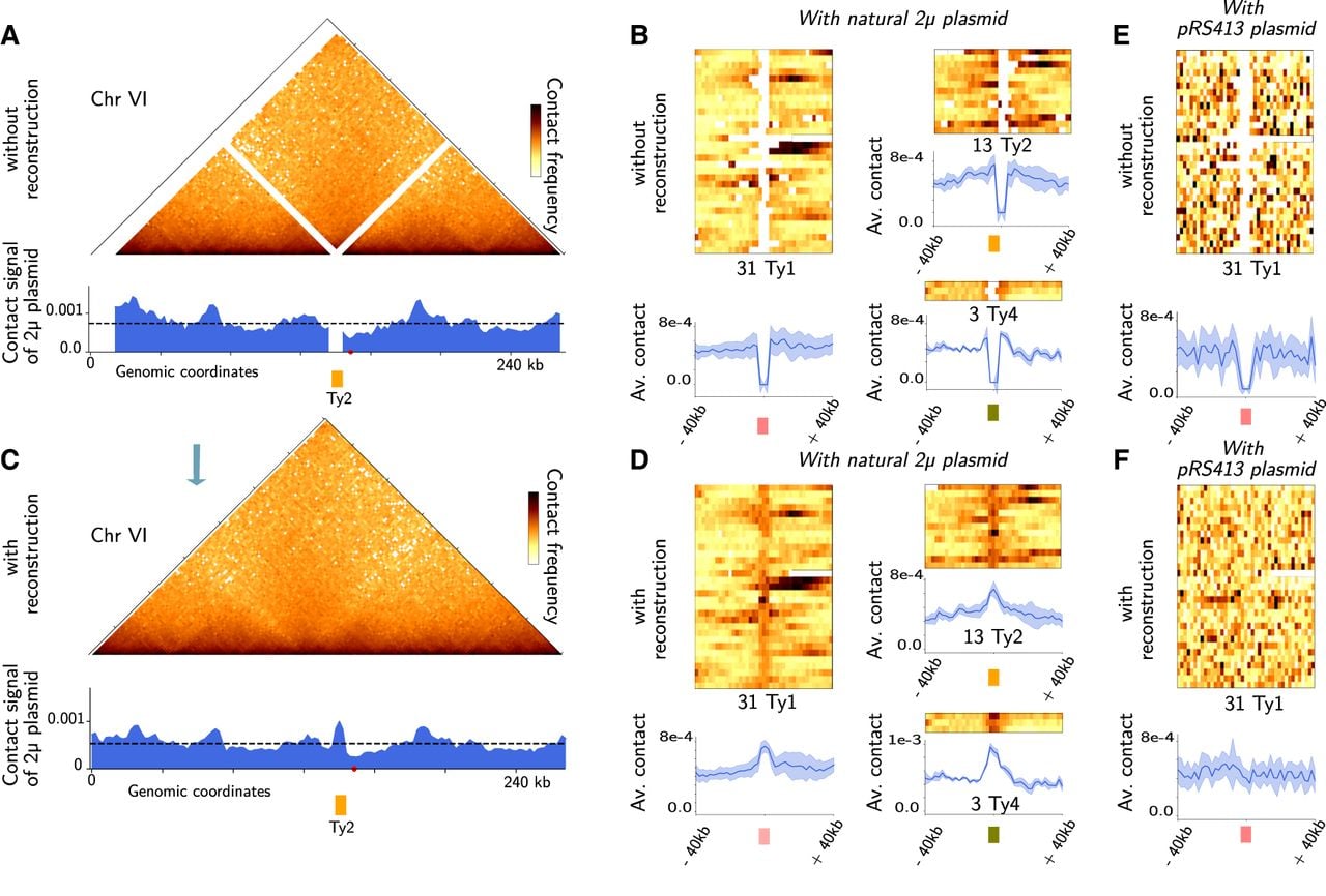
The average contact profile for each of the families shows contact enrichment. For the negative control, the same analysis was performed with the pR413 plasmid, which does not have the 2µ gluing system but relies on a centromeric system for its partitioning mechanism, and the contact enrichment is not present (Fig. 5E–F). This is also the case for other sequences used as negative controls: The mitochondria or other chromosomes of the host do not show enrichment with these same families of retrotransposons. It should be noted that even if the reconstructions for each specific retrotransposon are not necessarily perfect, their average signal should be correct. Therefore, the observation of the contact enrichment of the two-micron plasmid in association with retrotransposon families should be valid regardless of the accuracy of the reassignments. Interestingly, these reconstructions show that these two biological objects, the 2µ plasmid and Ty retrotransposons, which are in a sense two colonizers of the S. cerevisiae genome, co-locate inside the nucleus.
Cohesin can accumulate at the ends of Ty transposons
Chromosomal loops have recently been shown to form at certain stages of the cell cycle in mammals (Abramo et al. 2019) as well as in the model organism S. cerevisiae (Lazar-Stefanita et al. 2017). In the yeast S. cerevisiae, loops of 10–15 kb are formed by cohesin complexes in the G2/M phase (Costantino et al. 2020, Dauban et al. 2020), and their size can be finely regulated by a set of dedicated proteins, such as Pds5 or Wapl (Bastié et al. 2022). Cohesin complexes, which are molecular motors, can condense the whole genome, possibly through loop extrusion (Fudenberg et al. 2016), which can impact various biological processes such as DNA repair (Piazza et al. 2021). The minimum ingredients for the formation and precise positioning of these loops are still under debate. Some models, for example, have recently indicated that transcription is the source of energy that drives cohesin and engages it in chromosomal loops (Guérin et al. 2024). To explore the potential impact of the presence of retroposons on cohesin loop positioning, we produced reconstructions of chromosome Hi-C contact maps under two different biological conditions: In the G1 phase, cohesins are not bound to chromatin; and in the cdc20 genetic mutant, which synchronizes cells in the G2/M phase, cohesins create chromosomal loops. The data used were extracted from Piazza et al. (2021) in the W303 genetic background with the T2T assembly genome (Methods). Interestingly, we observed that retrotransposons placed in a convergent configuration, such as two pairs on Chromosome IV, are associated with the presence of chromosomal loops only in the G2/M phase (Fig. 6A–D, black arrows). Interestingly, the genome of strain W303 contains a third pair of retrotransposons in a convergent configuration, which also shows a loop pattern at the convergence area of Ty (Supplemental Fig. S26).
Yeast transposons can be associated with the positioning of cohesin loops in the S. cerevisiae genome. (A,B) Zoomed view of the contact map of Chromosome IV of S. cerevisiae without and with Hicberg reconstruction; bin = 2 kb in a population synchronized in the G1 phase (W303 strain) (data from Piazza et al. 2021). (C,D) Zoomed contact map of Chromosome IV of S. cerevisiae without and with Hicberg reconstruction in a population synchronized in the G2/M phase (W303 strain, cdc20 mutant) (data from Piazza et al. 2021). (E,F) Cohesin occupancy signal from ChIP-seq of Scc1 in the G2/M phase without and with Hicberg reconstruction. The forward and reverse genes are represented by blue and red arrows, respectively. Retrotransposons are represented by orange arrows. The black triangles point to chromosomal loops that are only visible with Hicberg reconstruction and are associated with cohesin occupancy peaks (Scc1) at convergent transposons.
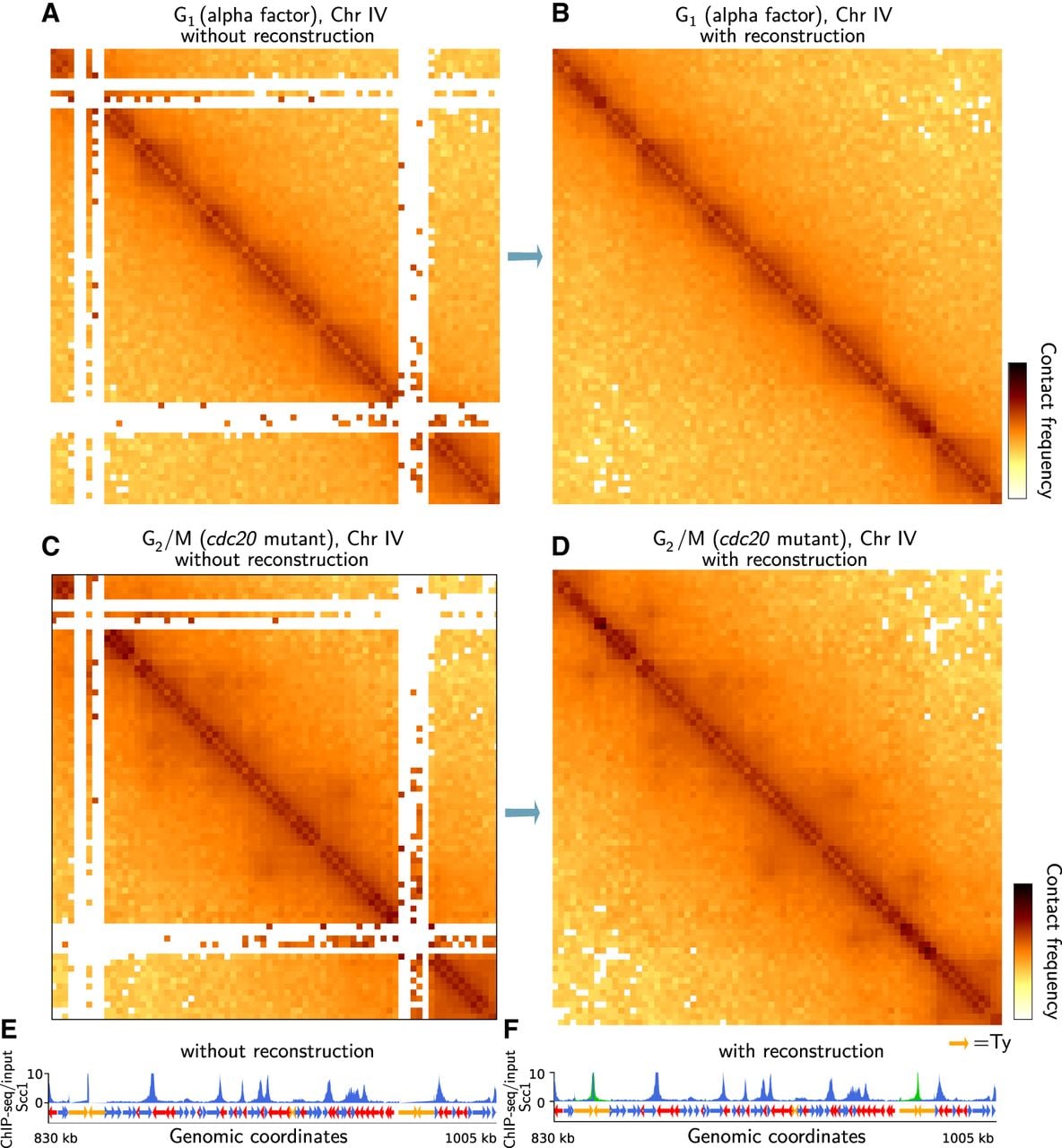
Although this is not its primary function and other algorithms perform this task, Hicberg can also be used to reconstruct 1D tracks of various genomic signals, such as nucleosome occupancy by MNase-seq (Supplemental Fig. S27; Guo et al. 2026), protein occupancy by ChIP-seq, or chromatin accessibility by ATAC-seq. To confront the chromosomal loops observed at the ends of Ty elements, we reconstructed the occupancy signal for the protein Scc1, which is part of the cohesin complex, and juxtaposed it with contact maps (Fig. 6E,F). Interestingly, we detected peaks of occupancy at the ends of the open reading frames (ORFs) of the Ty that form chromosomal loops. Notably, the peaks are sometimes already partially visible in the data without reconstruction.
To generalize the analysis, we constructed an agglomerated plot of the occupancy signal for the protein Scc1 for all Ty elements and for all genes of S. cerevisiae without and with Hicberg reconstruction. The Ty group is enriched at the ends of the ORF, which is more pronounced (a twofold increase) than the average of the yeast genes (Fig. 7A; for biological replicate, see Supplemental Fig. S28C; Chapard et al. 2025). When each family of retrotransposons is calculated separately (Supplemental Fig. S28A), this behavior is visible for the Ty1, Ty2, and Ty4 transposon families. We replicated the analysis in the S288C genetic background, in which the retrotransposons are not all at the same positions, and obtained similar results.
Averaged signal of cohesin occupancy and agglomerated contact plot of the transposons (Ty) in the yeast S. cerevisiae genome. (A) Averaged signal of cohesin occupancy (ChIP-seq of Scc1) at genes and at Ty elements without and with Hicberg reconstruction in the yeast S. cerevisiae in the G2/M phases of the cell cycle. (B) Agglomerated contact plots of Ty in the G1 and G2/M phases of the cell cycle without and with Hicberg reconstruction in the yeast S. cerevisiae.
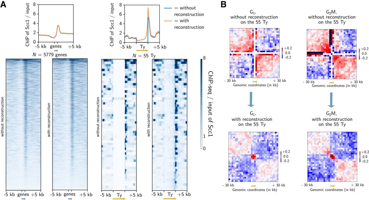
If we generate the average contact signal plot at the diagonal of the contact maps, we see a border pattern without and with reconstruction (Fig. 7B). Without reconstruction, the average plot contains fluctuations, but the border pattern is already visible with the presence of red squares on the diagonal and blue areas around them (contact depletion). The presence of a border pattern at the Ty regions during the G1 phase is quite unexpected, because these regions are not highly transcribed and cohesins are not functional at this stage of the cell cycle. Further experimental studies and analyses are needed to clarify the mechanisms underlying the presence of these patterns. The pattern also appears to be strongest in G2/M, when cohesin is active. With only reconstruction (Fig. 7B), the average plot shows a small area of the domain at the level of the Ty ORF, which has a size of ∼5.5 kb, namely, three bins, suggesting a structure linked to the Ty ORF, which is reminiscent of the gene globules observed in yeast in Micro-C (Hsieh et al. 2015; Hsieh et al. 2016). Finally, if we compute the average agglomerated signal between the different transposons, we do not detect any loop or enrichment pattern, indicating that the reconstructions do not show clustering of the different Ty within the nucleus (Supplemental Fig. S28B).
The Ty1 retrotransposons, which have been best characterized, are not known to have high transcriptional activity (but do have high RNA stability) under normal culture conditions (Curcio et al. 2015). The fact that they are associated with strong levels of cohesin occupancy at the ends of their ORF positions (twofold effect) is an intriguing observation in the context of understanding the ingredients required for the natural cohesin positioning throughout the cell cycle. Interestingly, cohesin has recently been shown to be enriched in the 5′ region of long interspersed nuclear element-1 (LINE-1 or L1), which is a retrotransposon group that constitutes 17% of the human genome (Li et al. 2024) and can form chromosomal loops between LINE-1 and their cognate gene promoters. All these observations suggest a potential impact of certain transposons, particularly long transposons, on the positioning of the molecular motors that organize genomes, such as cohesins.
Discussion
In this work, we present Hicberg, an algorithm based on statistical inference with the computation of specific probability distributions to reassign the positions of reads from repeated sequences. To the best of our knowledge, Hicberg is the only computational method that allows the positions of multimapping reads to be reattributed at all spatial scales. The algorithm does not filter the data and reconstructs all the events present in the high-throughput sequencing library in the pair ends, whether they are informative events, noninformative events or noise. This approach therefore enables the data to be reconstructed faithfully and can then be used to work on data that are more homogeneous across the whole genome. We demonstrated that our tool outperformed the only algorithm currently available for carrying out such an operation (mHi-C) (Zheng et al. 2019). Hicberg paves the way for the exploration of the functional 3D organization of repeated elements. It has been designed to be versatile and usable both for all Hi-C-derivative technologies and for a plethora of pair-ended omic data, as well as for a wide range of genomes and experimental conditions.
A current limitation of Hicberg reconstructions concerns regions with very low signals and high inhomogeneity, such as contact maps between different chromosomes. Our approach is sometimes unable to reconstruct the inhomogeneity of data around centromeric regions in particular. A possible extension would be to add a new level of information containing 2D signal variations, for example, via geometric extrapolations. Although such a refinement is possible and is currently being explored (density mode in the code), it presents a significant computational overhead that does not justify its implementation in the current Hicberg package. Indeed, the fact that Hicberg is capable of reconstructing signals that deviate from the average behavior, such as chromosome loops during certain cell cycle states or compartment signals, shows that the constraints provided by the reads present in the library and the statistical inference currently implemented in Hicberg are sufficient for the reconstruction of this type of signal.
One current area for improvement in the algorithm is reducing its computation time especially for organisms with families of repetitive sequences containing a large number of elements. The most time-consuming step in the algorithm is the reassignment of reads based on the defined probability distributions. To select an alignment from a distribution of possible alignments with different probabilities, we use the “random.choice” function from the “numpy” package. This function generates a random sample from a given 1D array of size N. Computing time is thus proportional to the number of probabilities N. The dominant factor is the path of the probability vector used to construct the cumulative distribution function (CDF). The computation time increases linearly with the size of the vector of probabilities. Because the probability distribution is not exactly the same for every pair of reads, the CDF must be computed for each read. Although it is possible to reconstruct Hi-C data from the human genome, particularly by limiting the number of possible alignments to 10,000. Computation times are on the order of a hundred hours for a standard machine, which currently prevents its everyday use in this context.
Furthermore, the use of Hicberg on contact data from strains whose genetic background could vary slightly from the reference genome resulted in the formation of unusual patterns on the contact maps, suggesting changes in the positions of repeated elements within these strains (Supplemental Fig. S22). Because Hicberg is sensitive to variations in genetic background, for example, positions of transposons, it can be used as an alternative tool for detecting genomic variations.
It should also be noted that Hi-C technologies coupled with long-read sequencing such as Nanopore are being developed, such as Pore-C (Zhong et al. 2023). However, these technologies need sufficient coverage (at least 200 million contact events) to achieve interesting resolutions at the genome scale.
Furthermore, although the read size with this type of sequencing reaches 5 kb, the reads are chimeric and contain several restriction fragments (which are ∼300 bp in size), which makes their mappability still insufficient for many families of repeated sequences and makes an approach such as Hicberg relevant.
With the growing appeal of chromosome contact techniques, driven by lower sequencing costs and optimized capture methods, the Hicberg algorithm provides a bioinformatic framework for the exploration of new hypotheses concerning genome architecture and the role of repeated elements.
Methods
Read alignment and classification
The alignment of reads to a reference genome was performed with Bowtie 2 (Langmead and Salzberg 2012) in the “very-sensitive-local” mode. For short-read Illumina Hi-C libraries, Bowtie 2 was chosen as the default aligner because several benchmarks report that it is generally faster and less memory intensive, while retaining high mapping accuracy for reads in the 50–150 bp range (Fonseca et al. 2012; Hatem et al. 2013). However, BWA-MEM may better rescue chimeric reads spanning ligation junctions via split-local alignment and can be used as well. For genomes containing repeated sequences with a reasonable number of occurrences (e.g., fewer than 4000), the -a option in Bowtie 2 can be used, which will give all possible positions for an ambiguous alignment, which is the case for the model organisms E. coli and S. cerevisiae. For genomes with many repeated sequences, the -k 100 option of Bowtie 2 could be used, resulting in 100 possible genomic positions for a read. The SAM files are then converted to BAM files via the software SAMtools (Li et al. 2009).
Computation of statistical trends
Different statistical trends are computed via uniquely mapping pairs to create a statistical model that is used to assign ambiguous reads. Here, we briefly describe the computations of two of them, but others can be generated and added to the model. We assume that each of the statistical trends is independent of the others.
– The statistical law known as P(s) represents the contact frequency as a function of the genomic distance s (in base pairs). This metric is regularly computed in Hi-C analyses. It contains a thermodynamic component: It derives from the polymer behavior of the chromosome, and the frequency of contact decreases as the genomic distance increases. It may also contain trends owing to biological chromatin condensation (e.g., during the G2/M phase of the cell cycle of the yeast S. cerevisiae, the appearance of regular loops every 15 kb has an impact on the behavior of this law) (Dauban et al. 2020).
Finally, this law also depends on the presence of noninformative events commonly present in the Hi-C libraries, which can be classified into three different categories and depend on the directionality of the reads that make up the pair (Matthey-Doret et al. 2022).
– “Dangling-ends” events correspond to nondigested collinear fragments that can represent a significant proportion of sequenced events in Hi-C libraries (with [+,−] orientations).
– “Self-circularized” events correspond to collinear fragments that have circularized on themselves (with [−,+] orientations).
– “Mirrors” events correspond to pairs of reads having the same orientation and aligning on the same restriction fragment (with [+,+] or [−,−] orientations).
We have therefore chosen to compute the P(s) law for each of these three possible configurations, namely, taking into account the directionality of the two reads making up the pair. This allows us to take advantage of the variability in the frequencies of appearance of these different types of events, presenting a discriminating property in the attribution of genomic coordinates for the multimapping read pairs (Supplemental Fig. S1A).
For contacts between different chromosomes, the average contact frequency for each pair of chromosomes is computed while accounting for the size of each of the two chromosomes.
– The second statistical trend we calculate is the coverage along the chromosomes. Each chromosome is binned at a given size (e.g., 2 kb), and the number of reads is counted for each bin. A smoothing procedure is applied via a sliding window. The window size is computed on the data by taking the maximum number of consecutive bins that have significantly low values (for which the number of reads is below the median − nmads × mad, where mad is the median absolute deviation; nmads by default is set to one).
Assignment of the contacts from the different possible pairs
Once these different trends have been computed, the propensity of each possible pair of reads (i,j) for the ambiguous alignments is computed as the product of the two previous statistical trends:
The propensities of possible contacts resulting from all (n,m) pair combinations are computed and form a probability law:
The function choice from the numpy.random package returns nonrepeated and nonuniform random samples of the given array F. Notably, the chosen coordinates are not necessarily those with the highest weight, which makes it possible to be more realistic about the statistical features of the data and allow for some fluctuations.
Generation of matrices and normalization
Pairs of contacts are then binned (by default, 2 kb bins) in contact matrices, which are normalized via the ICE method (Imakaev et al. 2012) and saved in the cool format (Abdennur and Mirny 2020).
Hicberg benchmarking
To quantify the quality of the reconstructions generated by Hicberg, we adopted a simulation strategy in which we controllably inject several possible alignments for a given genomic region. The first step is to define a set of genomic intervals whose number, genomic distance, or size can vary. Second, the set of (initially unambiguous) read pairs for which at least one of the two partners aligns with one of the previously defined genomic intervals is automatically duplicated in the set of other defined intervals in the alignment procedure (Supplemental Fig. S2).
Because the ambiguity injection procedure is performed under controlled and localized conditions, the quality of the reconstruction proposed by Hicberg is determined by comparing the bins (rows or columns of the contact matrix) relative to twin genomic regions between the initial matrix and the reconstruction resulting from Hicberg. The assessment of the reconstruction is then performed via the computation of Pearson's correlation of all the genomic bins affected by the injection of ambiguity between the initial vectors and the reconstruction given by Hicberg. This makes it possible to evaluate the closeness of the contact distribution between the initial signal and reconstruction. The closer this correlation coefficient is to one, the better the reconstruction is. To make this reconstruction score interpretable, we need to compare it with the score obtained via a null model, for which the pairs of twin genomic regions are randomly assigned. Each box plot corresponds to 20 different experiments.
For the performance benchmark, the standard data set used is a 47 million–read asynchronous S. cerevisiae Hi-C library generated with a standard protocol (Bastié et al. 2022). To compare the use of RAM memory and CPU computation time, this data set was sub-sampled to 1%, 10%, 25%, 50%, 75%, and 100%. Both Hicberg and mHi-C were tested in their respective standard modes, with the contact matrix resolution set at 2 kb. All programs were run with 16 CPU threads on an Intel Xeon W-2255 at 3.70 GHz and with 32 GB of RAM available. The software versions used for this benchmark were Hicberg v1.0.1 and the latest version of mHi-C available at GitHub (https://github.com/yezhengSTAT/mHiC) as of January 2025.
Generation and visualization of reconstructed contact maps
Chromosomal contact maps without and with reconstruction were normalized via the cooler package and visualized via Python code 2whole_matrices_reconstruction_mappability.py.
Theoretical mappability along the chromosomes was computed via the software GenMap (Pockrandt et al. 2020; https://github.com/cpockrandt/genmap with default parameters), and a BED file was generated for the plot with the contact map.
For the 4C-like signal for the telomeric region of the chimeric chromosome (Supplemental Fig. S25), the sum of the five last bins corresponding to the telomeric region was computed and then plotted along the chromosome (Python code: mycoT_4Clike.py).
Correlation matrices were calculated via the correlation_matrice.py code. Briefly, the data were normalized via the balance_cooler function in the cooler package. A detrending relative to the genomic distance was subsequently performed via the distance_law_from_mat function in the hicstuff package. Finally, the correlation matrix was computed via the corrcoef_sparse function in the hicstuff package.
Tys as 2µ plasmid contact hotspots
For the reconstruction of 2µ plasmid contact signal, a standard Hi-C library in log-phase condition was exploited, and the default parameters of Hicberg were used, as was the standard reference genome (sacCer3). The contact signal of the 2µ-plasmid was computed as previously described (Girard et al. 2025). Briefly, the 2µ plasmid contact signal is the number of contacts of the 2µ plasmid with a given bin (2 kb resolution) normalized by the number of Hi-C reads of the bin along the genome (to reduce the differences in detectability of certain regions) (Matthey-Doret et al. 2022) and divided by the proportion of reads coming from the 2µ sequence (to take into account differences in the number of copies of the plasmid for a given biological condition). The positions of the various transposons were extracted from the SGD database (http://sgd-archive.yeastgenome.org/sequence/S288C_reference/other_features/). Mean plots and contact heatmaps for each element of the different families were generated via the homemade Python code plasmid_HSC_1D_agglo.py.
Tys and cohesin positioning
Reconstruction of Hi-C maps and ChIP-seq of Scc1 protein data were performed with the default parameters of the Hicberg and W303 genomes from the T2T project (W303.asm01.HP0). Annotations of genes and Ty retrotransposons were performed via files from the gff3 annotation file (W303.asm01.HP0.mitochondrial_genome.tidy.gff3 from the https://www.evomicslab.org/db/ScRAPdb database).
The occupancy signals for Scc1 were reconstructed with the Hicberg default parameters of Hicberg in omics mode. BEDtools was used to convert pair files into BED files, and bedGraphToBigWig from the UCSC Genome Browser utilities was used to convert BED files to bigWig files. The occupancy signal representations for Scc1 for each element of the transposon families and their mean profile were produced via the deepTools tool suite (https://github.com/deeptools/deepTools).
Agglomerated contact plots of Ty elements were performed using the package hicue with extract mode and detrending (https://pypi.org/project/hicue/).
Identification of the position of transposons from contact signals
A 4C-like plot for a group of genomic elements was generated via custom-made Python codes available on GitHub (code: 4Clike_cool_multi.py); for example, for the group of transposons, at each position of the annotated Ty, the 4C-like signal was computed. The calculation of the 4C-like signal is similar to that of the 2µ plasmid contact signal; then, the total signal is summed. If other Ty elements are present, secondary peak(s) can be visualized.
Experimental confirmation of Ty presence
To validate the presence of an unannotated Ty in the reference genome at genomic position Chr 12: 818,200–818,800 bp, we designated primers on either side of the potential integration (primers used: PL-45 CACTGAAGTTAGTGCCCTTTATGG and PL-46 GGACGTCGGCATAATTGATGGAAC) via the DreamTaq PCR protocol. Sanger sequencing was also performed on the PCR products to confirm the presence of the transposon.
Code availability
The source code for Hicberg is available at GitHub (https://github.com/koszullab/Hicberg) and as Supplemental Code. All the scripts used to reproduce the figures and analyses are available at GitHub (https://github.com/axelcournac/Hicberg_bioanalysis).
Data access
All sequencing data generated in this study have been submitted to the NCBI BioProject database (https://www.ncbi.nlm.nih.gov/bioproject/) under accession number PRJNA1534974. All previously published data used in this study are publicly available, and their accession numbers are listed in Supplemental Table S1.
Competing interest statement
The authors declare no competing interests.
Acknowledgments
All the members of the Spatial Regulation of Genomes unit are thanked for stimulating discussions and feedback, especially Amaury Bignaud, Fabien Girard, and Jacques Sérizay. This work used the computational and storage services (TARS cluster) provided by the IT department at Institut Pasteur, Paris. We thank Stéphane Descorps Declere, Johann Dreo, Pascale Lesage, Nicolas Maillet, and Julien Mozziconacci for their stimulating discussions and Agnès Thierry for advice on the experimental section. The Inception program awarded S.G. a doctoral scholarship for the completion of his thesis. This research was supported by funding from the Agence Nationale de la Recherche JCJC program (ANR-19-CE45-0003) and DARRI INNOV 177-23 allocated to A.C.
Author contributions: S.G. and A.C. conceptualized the method. S.G. implemented the method in Python. S.G. and A.C. applied this method to the biological data. S.G. and A.C. interpreted the biological results. S.O. and M.D. helped with the code implementation. P.L. performed the experimental validation. S.G. and A.C. wrote the manuscript with feedback from all the authors. Supervision and funding acquisition were by A.C.
Footnotes
[1] Supplementary material [Supplemental material is available for this article.]
[2] Article published online before print. Article, supplemental material, and publication date are at https://www.genome.org/cgi/doi/10.1101/gr.281770.125.
[3] Freely available online through the Genome Research Open Access option.
References
- ↵Abdennur N, Mirny LA. 2020. Cooler: scalable storage for Hi-C data and other genomically labeled arrays. Bioinformatics 36: 311–316. 10.1093/bioinformatics/btz540
- ↵Abramo K, Valton AL, Venev SV, Ozadam H, Fox AN, Dekker J. 2019. A chromosome folding intermediate at the condensin-to-cohesin transition during telophase. Nat Cell Biol 21: 1393–1402. 10.1038/s41556-019-0406-2
- ↵Bastié N, Chapard C, Dauban L, Gadal O, Beckouët F, Koszul R. 2022. Smc3 acetylation, Pd5 and Scc2 control the translocase activity that establishes cohesin-dependent chromatin loops. Nat Struct Mol Biol 29: 575–585. 10.1038/s41594-022-00780-0
- ↵Bignaud A, Cockram C, Borde C, Groseille J, Allemand E, Thierry A, Marbouty M, Mozziconacci J, Espéli O, Koszul R. 2024. Transcription-induced domains form the elementary constraining building blocks of bacterial chromosomes. Nat Struct Mol Biol 31: 489–497. 10.1038/s41594-023-01178-2
- ↵Bonnet A, Lesage P. 2021. Light and shadow on the mechanisms of integration site selection in yeast Ty retrotransposon families. Curr Genet 67: 347–357. 10.1007/s00294-021-01154-7
- ↵Bunnik EM, Cook KB, Varoquaux N, Batugedara G, Prudhomme J, Cort A, Shi L, Andolina C, Ross LS, Brady D, 2018. Changes in genome organization of parasite-specific gene families during the plasmodium transmission stages. Nat Commun 9: 1910. 10.1038/s41467-018-04295-5
- ↵Carron L, Morlot JB, Matthys V, Lesne A, Mozziconacci J. 2019. Boost-HiC: computational enhancement of long-range contacts in chromosomal contact maps. Bioinformatics 35: 2724–2729. 10.1093/bioinformatics/bty1059
- ↵Chakraborty A, Wang JG, Ay F. 2022. dcHiC detects differential compartments across multiple Hi-C datasets. Nat Commun 13: 6827. 10.1038/s41467-022-34626-6
- ↵Chan KM, Liu YT, Ma CH, Jayaram M, Sau S. 2013. The 2 micron plasmid of Saccharomyces cerevisiae: a miniaturized selfish genome with optimized functional competence. Plasmid 70: 2–17. 10.1016/j.plasmid.2013.03.001
- ↵Chapard C, Bastié N, Cournac A, Chaptal L, Mboumba H, Queille S, Thierry A, Gadal O, Lengronne A, Koszul R, 2025. RNA Pol II-based regulations of chromosome folding. Cell Genom 5: 100970. 10.1016/j.xgen.2025.100970
- ↵Cockram C, Thierry A, Gorlas A, Lestini R, Koszul R. 2021. Euryarchaeal genomes are folded into SMC-dependent loops and domains, but lack transcription-mediated compartmentalization. Mol Cell 81: 459–472.e10. 10.1016/j.molcel.2020.12.013
- ↵Costantino L, Hsieh THS, Lamothe R, Darzacq X, Koshland D. 2020. Cohesin residency determines chromatin loop patterns. eLife 9: e59889. 10.7554/eLife.59889
- ↵Cournac A, Marie-Nelly H, Marbouty M, Koszul R, Mozziconacci J. 2012. Normalization of a chromosomal contact map. BMC Genomics 13: 436. 10.1186/1471-2164-13-436
- ↵Cournac A, Koszul R, Mozziconacci J. 2016. The 3D folding of metazoan genomes correlates with the association of similar repetitive elements. Nucleic Acids Res 44: 245–255. 10.1093/nar/gkv1292
- ↵Curcio MJ, Lutz S, Lesage P. 2015. The Ty1 LTR-retrotransposon of budding yeast, Saccharomyces cerevisiae. Microbiol Spectr 3: 1–35. 10.1128/microbiolspec.MDNA3-0053-2014
- ↵Dauban L, Montagne R, Thierry A, Lazar-Stefanita L, Bastié N, Gadal O, Cournac A, Koszul R, Beckouët F. 2020. Regulation of cohesin-mediated chromosome folding by Eco1 and other partners. Mol Cell 77: 1279–1293.e4. 10.1016/j.molcel.2020.01.019
- ↵Dekker J, Mirny LA. 2024. The chromosome folding problem and how cells solve it. Cell 187: 6424–6450. 10.1016/j.cell.2024.10.026
- ↵Dekker J, Rippe K, Dekker M, Kleckner N. 2002. Capturing chromosome conformation. Science 295: 1306–1311. 10.1126/science.1067799
- ↵Dekker J, Marti-Renom MA, Mirny LA. 2013. Exploring the three-dimensional organization of genomes: interpreting chromatin interaction data. Nat Rev Genet 14: 390–403. 10.1038/nrg3454
- ↵Fang K, Wang J, Liu L, Jin VX. 2022. Mapping nucleosome and chromatin architectures: a survey of computational methods. Comput Struct Biotechnol J 20: 3955–3962. 10.1016/j.csbj.2022.07.037
- ↵Fleetwood DJ, Khan AK, Johnson RD, Young CA, Mittal S, Wrenn RE, Hesse U, Foster SJ, Schardl CL, Scott B. 2011. Abundant degenerate miniature inverted-repeat transposable elements in genomes of epichloid fungal endophytes of grasses. Genome Biol Evol 3: 1253–1264. 10.1093/gbe/evr098
- ↵Fonseca NA, Rung J, Brazma A, Marioni JC. 2012. Tools for mapping high-throughput sequencing data. Bioinformatics 28: 3169–3177. 10.1093/bioinformatics/bts605
- ↵Forcato M, Nicoletti C, Pal K, Livi CM, Ferrari F, Bicciato S. 2017. Comparison of computational methods for Hi-C data analysis. Nat Methods 14: 679–685. 10.1038/nmeth.4325
- ↵Fudenberg G, Imakaev M, Lu C, Goloborodko A, Abdennur N, Mirny LA. 2016. Formation of chromosomal domains by loop extrusion. Cell Rep 15: 2038–2049. 10.1016/j.celrep.2016.04.085
- ↵Girard F, Even A, Thierry A, Ruault M, Meneu L, Larrous P, Garnier M, Adiba S, Taddei A, Koszul R, et al. 2025. Parasitic plasmids are anchored to inactive regions of eukaryotic chromosomes through a nucleosome signal. EMBO J 44: 2134–2156. 10.1038/s44318-025-00389-1
- ↵Guérin TM, Barrington C, Pobegalov G, Molodtsov MI, Uhlmann F. 2024. An extrinsic motor directs chromatin loop formation by cohesin. EMBO J 43: 4173–4196. 10.1038/s44318-024-00202-5
- ↵Guidi M, Ruault M, Marbouty M, Loïodice I, Cournac A, Billaudeau C, Hocher A, Mozziconacci J, Koszul R, Taddei A. 2015. Spatial reorganization of telomeres in long-lived quiescent cells. Genome Biol 16: 206. 10.1186/s13059-015-0766-2
- ↵Guo X, Alhussain MM, Lee B, Byrne N, Hokamp K, Aljaeed H, Alnajjar RH, Baazeem ZMF, Smethurst G, Kröger C, 2026. Context-dependent interplay of Swi-Snf and Tup1-Cyc8 influences chromatin and transcription at antagonistically regulated genes. Nat Commun 17: 8134. 10.1038/s41467-026-74863-7
- ↵Hatem A, Bozdağ D, Toland AE, Çatalyürek ÜV. 2013. Benchmarking short sequence mapping tools. BMC Bioinformatics 14: 184. 10.1186/1471-2105-14-184
- ↵Hsieh THS, Weiner A, Lajoie B, Dekker J, Friedman N, Rando OJ. 2015. Mapping nucleosome resolution chromosome folding in yeast by Micro-C. Cell 162: 108–119. 10.1016/j.cell.2015.05.048
- ↵Hsieh THS, Fudenberg G, Goloborodko A, Rando OJ. 2016. Micro-C XL: assaying chromosome conformation from the nucleosome to the entire genome. Nat Methods 13: 1009–1011. 10.1038/nmeth.4025
- ↵Hu Y, Ma W. 2021. EnHiC: learning fine-resolution Hi-C contact maps using a generative adversarial framework. Bioinformatics 37: i272–i279. 10.1093/bioinformatics/btab272
- ↵Imakaev M, Fudenberg G, McCord RP, Naumova N, Goloborodko A, Lajoie BR, Dekker J, Mirny LA. 2012. Iterative correction of Hi-C data reveals hallmarks of chromosome organization. Nat Methods 9: 999–1003. 10.1038/nmeth.2148
- ↵Karpinska MA, Zhu Y, Fakhraei Ghazvini Z, Ramasamy S, Barbieri M, Cao TBN, Varahram N, Aljahani A, Lidschreiber M, Papantonis A, 2025. CTCF depletion decouples enhancer-mediated gene activation from chromatin hub formation. Nat Struct Mol Biol 32: 1268–1281. 10.1038/s41594-025-01555-z
- ↵Langmead B, Salzberg SL. 2012. Fast gapped-read alignment with Bowtie 2. Nat Methods 9: 357–359. 10.1038/nmeth.1923
- ↵Lazar-Stefanita L, Scolari VF, Mercy G, Muller H, Guérin TM, Thierry A, Mozziconacci J, Koszul R. 2017. Cohesins and condensins orchestrate the 4D dynamics of yeast chromosomes during the cell cycle. EMBO J 36: 2684–2697. 10.15252/embj.201797342
- ↵Lazar-Stefanita L, Luo J, Montagne R, Thierry A, Sun X, Mercy G, Mozziconacci J, Koszul R, Boeke JD. 2022. Karyotype engineering reveals spatio-temporal control of replication firing and gene contacts. Cell Genomics 2: 100163. 10.1016/j.xgen.2022.100163
- ↵Li H, Handsaker B, Wysoker A, Fennell T, Ruan J, Homer N, Marth G, Abecasis G, Durbin R, 1000 Genome Project Data Processing Subgroup. 2009. The Sequence Alignment/Map format and SAMtools. Bioinformatics 25: 2078–2079. 10.1093/bioinformatics/btp352
- ↵Li X, Bie L, Wang Y, Hong Y, Zhou Z, Fan Y, Yan X, Tao Y, Huang C, Zhang Y, 2024. LINE-1 transcription activates long-range gene expression. Nat Genet 56: 1494–1502. 10.1038/s41588-024-01789-5
- ↵Lieberman-Aiden E, Van Berkum NL, Williams L, Imakaev M, Ragoczy T, Telling A, Amit I, Lajoie BR, Sabo PJ, Dorschner MO, 2009. Comprehensive mapping of long-range interactions reveals folding principles of the human genome. Science 326: 289–293. 10.1126/science.1181369
- ↵Marin MA, Vicente ACP. 2013. Architecture of the superintegron in Vibrio cholerae: identification of core and unique genes. F1000Res 2: 63. 10.12688/f1000research.2-63.v1
- ↵Matthey-Doret C, Baudry L, Mortaza S, Moreau P, Koszul R, Cournac A. 2022. Normalization of chromosome contact maps: matrix balancing and visualization. Methods Mol Biol 2301: 1–15. 10.1007/978-1-0716-1390-0_1
- ↵McQuaid ME, Mereshchuk A, Dobson MJ. 2019. Insights into the DNA sequence elements required for partitioning and copy number control of the yeast 2-micron plasmid. Curr Genet 65: 887–892. 10.1007/s00294-019-00958-y
- ↵Meneu L, Chapard C, Serizay J, Westbrook A, Routhier E, Ruault M, Perrot M, Minakakis A, Girard F, Bignaud A, 2025. Sequence-dependent activity and compartmentalization of foreign DNA in a eukaryotic nucleus. Science 387: eadm9466. 10.1126/science.adm9466
- ↵Miao Z, Ren Y, Tarabini A, Yang L, Li H, Ye C, Liti G, Fischer G, Li J, Yue J-X. 2025. ScRAPdb: an integrated pan-omics database for the Saccharomyces cerevisiae reference assembly panel. Nucleic Acids Res 53: D852–D863. 10.1093/nar/gkae955
- ↵Morillon A, Bénard L, Springer M, Lesage P. 2002. Differential effects of chromatin and Gcn4 on the 50-fold range of expression among individual yeast Ty1 retrotransposons. Mol Cell Biol 22: 2078–2088. 10.1128/MCB.22.7.2078-2088.2002
- ↵O'Donnell S, Yue JX, Saada OA, Agier N, Caradec C, Cokelaer T, De Chiara M, Delmas S, Dutreux F, Fournier T, 2023. Telomere-to-telomere assemblies of 142 strains characterize the genome structural landscape in Saccharomyces cerevisiae. Nat Genet 55: 1390–1399. 10.1038/s41588-023-01459-y
- ↵Piazza A, Bordelet H, Dumont A, Thierry A, Savocco J, Girard F, Koszul R. 2021. Cohesin regulates homology search during recombinational DNA repair. Nat Cell Biol 23: 1176–1186. 10.1038/s41556-021-00783-x
- ↵Piveteau V, Dupont C, Salari H, Dumont A, Savocco J, Jost D, Piazza A. 2026. Condensin loop extrusion properties, roadblocks, and role in homology search during recombination in S. cerevisiae. EMBO J 45: 3124–3155. 10.1038/s44318-026-00748-6
- ↵Pockrandt C, Alzamel M, Iliopoulos CS, Reinert K. 2020. GenMap: ultra-fast computation of genome mappability. Bioinformatics 36: 3687–3692. 10.1093/bioinformatics/btaa222
- ↵Rippe K. 2001. Making contacts on a nucleic acid polymer. Trends Biochem Sci 26: 733–740. 10.1016/S0968-0004(01)01978-8
- ↵Rowe-Magnus DA, Guérout AM, Mazel D. 1999. Super-integrons. Res Microbiol 150: 641–651. 10.1016/S0923-2508(99)00127-8
- ↵Ruault M, Scolari VF, Lazar-Stefanita L, Hocher A, Loïodice I, Koszul R, Taddei A. 2021. Sir3 mediates long-range chromosome interactions in budding yeast. Genome Res 31: 411–425. 10.1101/gr.267872.120
- ↵Sau S, Ghosh SK, Liu YT, Ma CH, Jayaram M. 2019. Hitchhiking on chromosomes: a persistence strategy shared by diverse selfish DNA elements. Plasmid 102: 19–28. 10.1016/j.plasmid.2019.01.004
- ↵Thiaucourt F, Manso-Silvan L, Salah W, Barbe V, Vacherie B, Jacob D, Breton M, Dupuy V, Lomenech AM, Blanchard A, 2011. Mycoplasma mycoides, from “mycoides small colony” to “capri”: a microevolutionary perspective. BMC Genomics 12: 114. 10.1186/1471-2164-12-114
- ↵Wang M, Sunkel BD, Ray WC, Stanton BZ. 2022. Chromatin structure in cancer. BMC Mol Cell Biol 23: 35. 10.1186/s12860-022-00433-6
- ↵Wei Y, Ho YC. 2022. Interferon opens up: HIV-induced inflammation reconfigures 3D chromatin conformation and affects where HIV integrates. Mol Cell 82: 4585–4587. 10.1016/j.molcel.2022.11.013
- ↵Winter DJ, Ganley ARD, Young CA, Liachko I, Schardl CL, Dupont PY, Berry D, Ram A, Scott B, Cox MP. 2018. Repeat elements organise 3D genome structure and mediate transcription in the filamentous fungus Epichloë festucae. PLoS Genet 14: e1007467. 10.1371/journal.pgen.1007467
- ↵Yang JH, Hansen AS. 2024. Enhancer selectivity in space and time: from enhancer–promoter interactions to promoter activation. Nat Rev Mol Cell Biol 25: 574–591. 10.1038/s41580-024-00710-6
- ↵Zhang Y, An L, Xu J, Zhang B, Zheng WJ, Hu M, Tang J, Yue F. 2018. Enhancing Hi-C data resolution with deep convolutional neural network HiCPlus. Nat Commun 9: 750. 10.1038/s41467-018-03113-2
- ↵Zhang Y, Li T, Preissl S, Amaral ML, Grinstein JD, Farah EN, Destici E, Qiu Y, Hu R, 2019. Transcriptionally active HERV-H retrotransposons demarcate topologically associating domains in human pluripotent stem cells. Nat Genet 51: 1380–1388. 10.1038/s41588-019-0479-7
- ↵Zheng Y, Ay F, Keles S. 2019. Generative modeling of multimapping reads with mHi-C advances analysis of Hi-C studies. eLife 8: e38070. 10.7554/eLife.38070
- ↵Zhong JY, Niu L, Lin ZB, Bai X, Chen Y, Luo F, Hou C, Xiao CL. 2023. High-throughput Pore-C reveals the single-allele topology and cell type-specificity of 3D genome folding. Nat Commun 14: 1250. 10.1038/s41467-023-36899-x