Statistically rigorous and computationally efficient chromatin stripe detection with Quagga

Quagga overview

Quagga is a chromatin stripe detection tool that determines chromosomal coordinates that form an accurate bounding box around detected chromatin stripes. It works on all 3C family sequencing types, including Hi-C, Micro-C, and HiChIP. Quagga uses two major steps to find chromatin stripes. First, Quagga performs a quick screening of potential stripes and determines stripe width. Second, using the potential stripe list, Quagga checks for statistical enrichment and determines the stripe's length (Fig. 1A).

Figure 1.

Quagga is a lightweight tool that calls architectural stripes from a 3C chromatin contact frequency matrix. (A) The workflow of Quagga. (B) A 3C family-type contact frequency matrix via a COOL or HIC file is processed into a horizontally or vertically loaded matrix, and a naive peak-finding algorithm is used; stripe indices and width are calculated based on the vertically or horizontally averaged row or column sums. (C) Significance testing is applied to the candidate stripes from the previous step. Called region windows are used to determine the appropriate length of the stripe and whether the stripe is enriched over the local background.

Open in new tabDownload PowerPointLink to figure

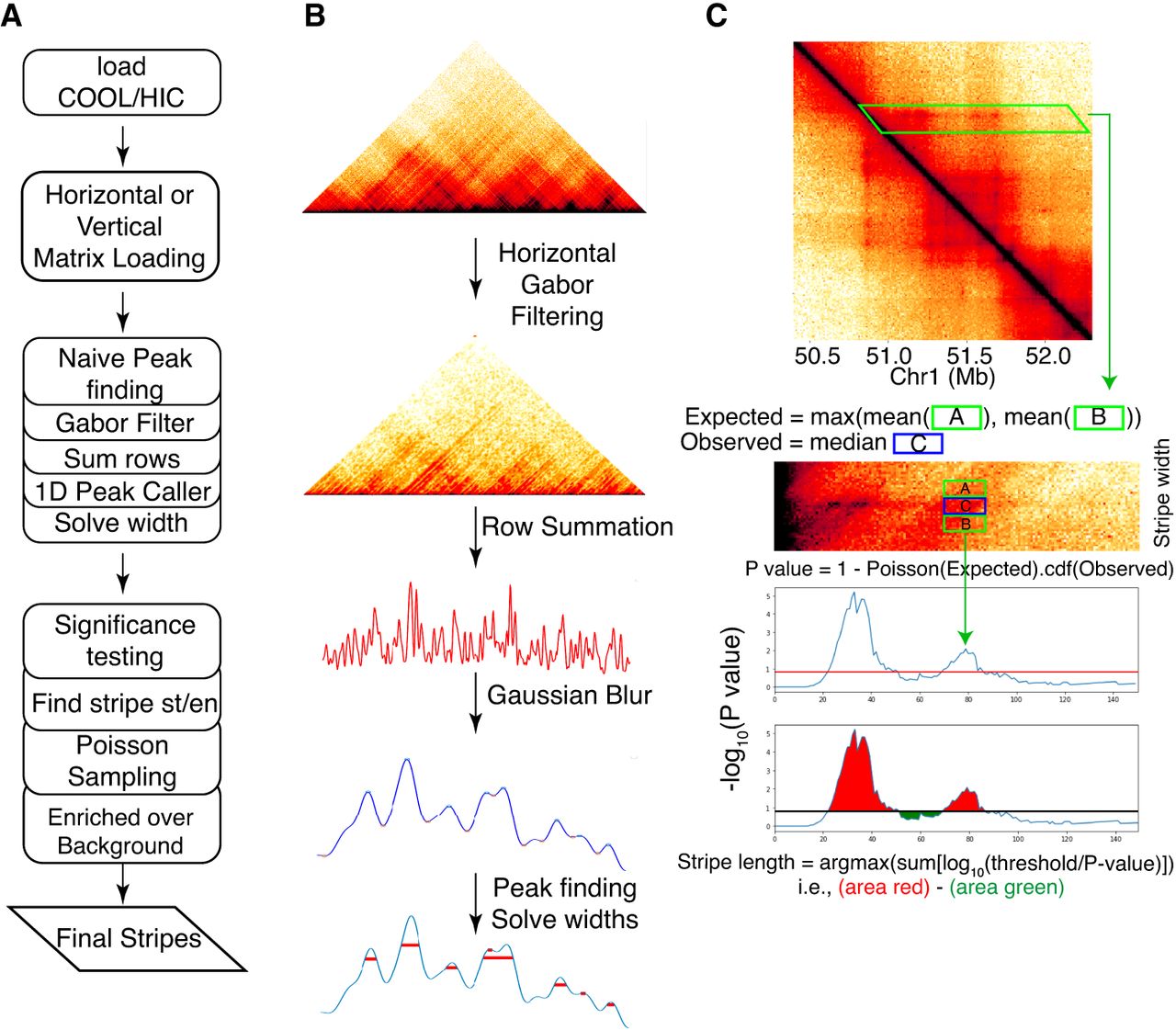
Quagga uses signal processing techniques to perform naive stripe calling and determine width. First, it reduces the chromosome into 5′ or 3′ signal vectors. A vertical or horizontal loading matrix is filled, taking a maximum length along the 5′ or 3′ direction on the contact frequency matrix. For example, a horizontal loading matrix has its rows containing the values of the rows of the corresponding coordinates of the contact frequency matrix, starting from the main diagonal and out to the maximum distance specified. A vertical loading matrix is filled similarly, in which its rows are filled with the columns of the contact frequency matrix instead. Then Quagga filters the loading matrices using a Gabor kernel Granlund (1978) to focus the angular signal from the underlying image. This strategy emphasizes high-contrast lines instead of dots or spots, which reduces noise and avoids single loops being called. Then the loading matrices are summed over their rows to form a 1D signal vector that reflects the signal buildup over its respective axis; the intuition is that major anchors will accumulate a tremendous amount of contact frequency signal and that nonstripe loop or TAD interactions can be filtered out in statistical enrichment. We apply Gaussian blur to reduce the noise of the vector and run a 1D peak-finding algorithm to determine local maxima and their widths (Fig. 1B) as our naive stripes.

Quagga next checks all stripes to determine appropriate stripe calls and assigns stripes a length. To do this, Quagga calculates a P-value for each pixel along the candidate stripes based on Poisson statistics by comparing observed to expected chromatin contact frequency (Fig. 1C). The observed value is determined along the length of the naive stripe using the solved width; expected values are based on windows flanking the stripe area. Using the P-values solved along the length of the stripe, Quagga uses a simple maximization calculation to determine the most likely starting and ending positions. In this way, an integrity score like Stripenn's stripiness is not necessary as Quagga already checks for stripe integrity by maximizing the significance of the observed stripe over the expected signal based on its neighbors.

Quagga efficiently detects stripes across diverse cell types, sequencing depths, resolutions, and 3C methods

We applied Quagga to call stripes from Hi-C contact maps of different cell lines. Quagga found 4133 stripes for GM12878 at 10 kb resolution, 10,398 for H1, 2908 for K562, and 8189 for HFFc6, respectively (Supplemental Fig. 1). Similar to Hi-C loop callers, Quagga calls are also dependent on sequencing depth and resolution. On a standard Hi-C GM12878 data set (Rao et al. 2014), we tested a range of sequencing depths from 4 billion filtered read pairs to as low as 15.6 million filtered read pairs and found Hi-C data stripe detection effective at 250 million filtered reads or more (Supplemental Figs. 2, 3). Quagga was consistent between 5 kb and 10 kb resolution calls; Quagga identified fewer stripes at 5 kb resolution, and these stripes also tended to be shorter in length. We believe this is because of increased sparsity in the contact maps at higher resolution (Supplemental Fig. 4). In particular, longer-range interactions become even sparser owing to distance-dependent contact decay, making it less likely for stripes to be detected over longer genomic distances.

Quagga's stripe calls were also consistent between biological replicates. Of stripes found by Quagga, 673 of 1167 were unique in bioreplicate 1 (Rep1) and 344 of 837 were unique in bioreplicate 2 (Rep2), which for shared stripes between the two replicates is 42.3% and 58.9%, respectively (Supplemental Fig. 5A).

Quagga can also be applied to additional 3C data, such as HiChIP. We found 3782 stripes from HiChIP in SMC1 and 2970 stripes in CTCF (Supplemental Table 1). We also attempted to call Quagga on split-pool recognition of interactions by tag extension data (SPRITE); however, because of the differences in the underlying chemistry, Quagga required hand annotation to find true-positive stripes (Supplemental Fig. 6).

Quagga is also algorithmically efficient. For stripe calling from GM12878 Hi-C data, Quagga required 99 min compared with 65 min for Zebra and 505 min for Stripenn. In all tools, the primary time-consuming step is statistical significance testing, as more stripe candidates lead to more significance assessments. Despite performing substantially more statistical tests, Quagga completes its runs within a reasonable timeframe.

Stripes called by Quagga have the most variety and match size-scale

We demonstrate the ability of Quagga to detect stripes from Hi-C contact maps by aggregating the various sizes of all called stripes of Quagga, Stripenn, and Zebra. These stripes are based on the same publicly available GM12878 Hi-C data at 10 kb resolution calls on the whole genome. Quagga called 4133 stripes, Zebra called 3278 stripes, and Stripenn called 873 stripes (Fig. 2A). A considerable number of each tool's stripes are unique, but many are also shared (Supplemental Fig. 7). Looking at tool-exclusive stripes, Quagga found 2702, Zebra 1826, and Stripenn 169 stripes, for which Quagga-only stripes have the highest enrichment of CTCF binding (Supplemental Fig. 8). To assess how reasonable the aggregates of each tool's stripe output were, we quantitatively examined the differences in their distribution of stripe lengths, stripe widths, and performed two kinds of pileup aggregated peak analysis (APA). We defined a reasonable distribution of peak lengths as one near the median CTCF/cohesin loop anchor span (300 kb) and at or below the median TAD sizes (500 kb) (Dixon et al. 2012; Fudenberg et al. 2016; Xi and Beer 2021). Quagga stripe lengths range mostly between 50 kb to 320 kb. Zebra's total span trended longer than Quagga's overall, but enough of the lengths appeared to be reasonable, whereas Stripenn's stripe lengths are normally distributed ∼1 Mb long (Fig. 2A). These results suggest that Quagga and Zebra are more sensitive to detecting shorter stripes than Stripenn. And although Zebra has a reasonable length distribution, there are a large number of false-positive stripes if we do not perform the additional steps of removing loops and TAD boundaries (for an example, see Fig. 2E and Supplemental Fig. 9). Stripe-width distributions between Quagga and Stripenn highlight Quagga's adaptability to capture many different widths in comparison to Stripenn (Fig. 2B). Zebra only provides the midpoint of the solved stripe coordinate, as all those stripes are uniformly reported as 10 kb wide.

Figure 2.

Benchmarking of three stripe callers, including Quagga, Zebra, and Stripenn, with Hi-C contact maps. (A) Quagga's stripe lengths lie mostly in the expected range compared with Stripenn or Zebra. (B) Stripe widths for Quagga are also the most varied. (C) Aggregated peak pileups using a 2 Mb window centered on the point of the main diagonal nearest the stripe's anchor, which demonstrates the high variability of the stripe length and width Quagga captures. (D) Scaled Quagga pileups along the entire stripe length show Quagga's variability and distribution of stripes; the beginning of the stripe is fixed to the start position, and half its length in either direction is captured as a context sequence. (E) Examples of stripes called by Quagga, Zebra, and Stripenn from GM12878 Hi-C.

Open in new tabDownload PowerPointLink to figure

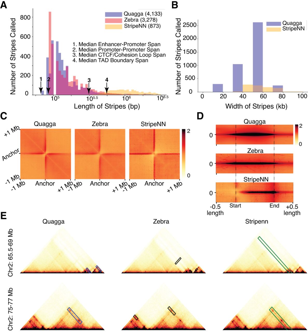
APA pileup using stripe coordinates on the source Hi-C data (Fig. 2C) demonstrates the uniformity of stripe calls in Stripenn, while showing that a variety of signal widths and lengths are in Quagga and Zebra, evident by the tapering pileup. This analysis underlines Quagga's versatility in comparison to the other tools, evident by the longer, wider, and nonuniform pileup that captures a very wide variety of stripe lengths and widths. Tool-unique stripe APAs demonstrate Stripenn has a stark, block appearance, along with Stripenn's high count of long stripes, suggesting many counts may be TADs (Supplemental Fig. 8). Finally, a dynamically scaled APA pileup along the length of stripes per tool shows the relative contact signals along the stripes (Fig. 2D). As all signal is captured in these length-scaled windows, the presence of signal before the starting line is expected, as this should include the main diagonal or other elements in line with the stripe that are not captured. Stripenn always starts at the main diagonal, so no leading signal would be counted before the start point.

Quagga identifies the close connection between Hi-C stripes and CTCF/cohesin binding

The Hi-C stripe formation is commonly explained with one-sided extrusion. Therefore, we investigated the CTCF/RAD21 binding pattern of stripe anchors to assess Quagga's outputs. In the GM12878 Hi-C contact map, Quagga identified 4133 stripes at 10 kb resolution. Quagga-identified stripes are further categorized into two groups: 3′ stripes spanning downstream and 5′ stripes spanning upstream. We analyzed CTCF/RAD21 enrichment and CTCF orientation patterns at Quagga-called stripes, with the binding sites identified from ChIP-seq data and CTCF orientations annotated based on the underlying DNA sequence motifs. Our analysis revealed a significant enrichment of CTCF and RAD21 at both 3′ and 5′ stripe anchors identified by Quagga, signifying the dominance of extrusion-based stripes (Fig. 3A,B).

Figure 3.

Hi-C stripes called by Quagga are closely related to CTCF/RAD21 extrusion. For both 3′ and 5′ stripes, CTCF (A) and RAD21 (B) are enriched at GM12878 stripe anchors. (C) Quagga detects four times stripes as Stripenn and demonstrates the same CTCF enrichment pattern compared with Stripenn, in which 5′ stripe anchors are more enriched in positive-strand CTCF, and the 3′ stripes are more enriched in negative-strand CTCF.

Open in new tabDownload PowerPointLink to figure

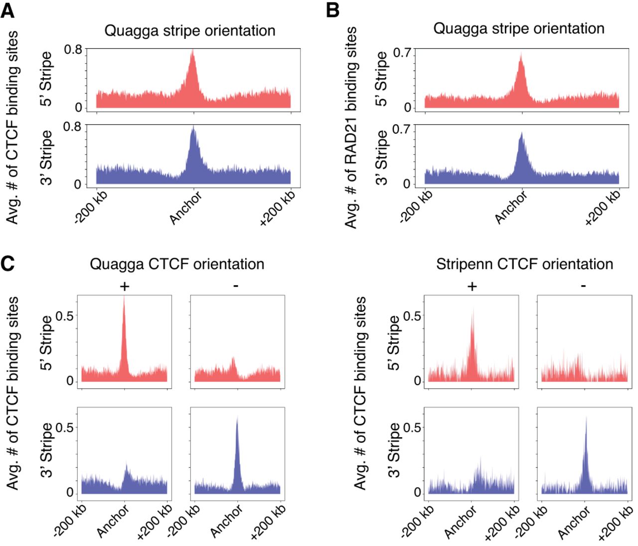
We also detect distinct patterns of CTCF orientation for the two stripe groups. Specifically, the 3′ stripes exhibited a significant enrichment of forward-strand (+) CTCF orientations and a depletion of backward-strand (−) CTCF orientations, with the reverse being true for the 5′ stripes (Fig. 3C). As a comparison, stripes called by the baseline method Stripenn are less enriched in CTCF binding (Fig. 3C). This observation demonstrates that Quagga effectively identifies the prototypical CTCF/RAD21-extrusion stripes in Hi-C data.

Our assessment of CTCF-stripe assignment is supported by performing stripe calls on auxin-induced CTCF degradation, a technique for loop knockdown. Quagga called 3873 stripes on the control compared with 55 in the auxin-treated sample, strongly indicative that CTCF-loops play an outsize role in chromatin stripe formation (Supplemental Fig. 10).

Quagga calls more CTCF-stripes and has the least indeterminate stripes

To assess the quality of chromatin stripes found using Quagga, Zebra, and Stripenn, we sought to classify our stripes into three categories, namely (1) CTCF-motif occupied by CTCF-stripes, “CTCF-stripes”; (2) CTCF-deficient stripes that intersect with EP-interacting regions, “EP-stripes”; and (3) CTCF-deficient stripes that are not EP-intersecting, “indeterminate.” We follow the convention of previous studies in simplifying promoter–promoter (PP) and EP interactions both as EP interactions (Hsieh et al. 2022). From 4133 Quagga stripe calls, 87.83% were CTCF-occupied (3630), 2.6% were EP-stripes (110), and 9.5% indeterminate (393); of Zebra's 3278 stripes, 76.9% were CTCF-occupied (2523), 7.38% were EP-stripes (242), and 15.6% were indeterminate (513); and from Stripenn's 873 stripes, 84.5% were CTCF-occupied (738), 2.5% were EP-stripes (22), and 12.9% were indeterminate (113) (Fig. 4A; Supplemental Figs. 11, 12). Quagga and Zebra each found four to five times more stripes, respectively, than Stripenn. Quagga's number of called stripes on Hi-C data was the most numerous and by percentage the highest enriched in CTCF. Quagga has the lowest proportion of indeterminate calls, which, from our observation, are highly related to regions with low mappability or bad matrix normalization (Supplemental Fig. 11).

Figure 4.

Quagga, Stripenn, and Zebra were compared for their ability to reasonably call CTCF-anchored stripe based on stripe length, CTCF/RAD21 enrichment, and their proportion of off-target stripes found. (A) Distribution of CTCF-stripe lengths from stripes detected by Quagga, Zebra, and Stripenn. (B) Histogram depicting the frequency of stripe occurrence depending on the length of the found stripe for CTCF-anchored stripes. (C) Breakdown of our analysis for stripes belonging to CTCF-stripes, to stripes intersecting enhancer–promoter interacting annotated regions but not CTCF-occupied motifs (EP-stripes), and stripes that do not intersect with CTCF motifs or EP annotated regions (indeterminate-stripes). Indeterminate stripes may be false positives. Quagga best minimizes indeterminate stripes.

Open in new tabDownload PowerPointLink to figure

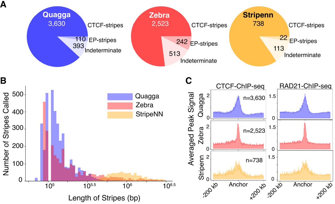
Classifiable stripe calls fall into either dynamic chromatin looping capture or EP interactions; therefore, we assess the quality of each stripe calling tool's outputs by examining if their lengths are reasonable, if CTCF-related stripes are enriched in CTCF/RAD21, and if the stripe calls are generally classifiable. To understand if a stripe length is reasonable, we consider that the median size for chromatin looping is 300 kb and that going beyond the median TAD boundary span of 500 kb would suggest a false positive (Hsieh et al. 2022). Quagga and Zebra's distributions of CTCF-occupied stripes align strongly with the expected spans, whereas Stripenn's CTCF-stripes trend longer than the median TAD span (Fig. 4B). Stripenn's trend toward longer stripes may suggest it confuses TAD bounds or compartments for stripes.

CTCF-stripes called by all methods are enriched in CTCF and RAD21, in which Quagga and Zebra's aggregated peak signal is strongest (Fig. 4C). Stripenn CTCF and RAD21 peaks are more dispersed and broader. We observe a similar concentrated pileup of CTCF and RAD21 of CTCF-stripes in our benchmarking experiments with downsampled contact maps (Supplemental Fig. 3B) and contact maps of biological replicates (Supplemental Fig. 5B,C). This indicates that Quagga's detection of CTCF-stripes is consistent across different conditions. The CTCF/RAD21 concentration is visible across 5 kb or 10 kb Hi-C resolution, and we observed higher enrichment of CTCF and active histone marks at 5 kb-detected stripes (Supplemental Fig. 4C), which may reflect a more accurate localization of stripe anchors at higher resolution.

Quagga EP-stripes have strong histone modification signal related to enhancer/promoter activity

Similar to for CTCF-stripes, we report each tool's capability for capturing EP or PP interactions, which for simplicity are termed EP-stripes. We designate EP-stripes as those stripes that, along their narrow width, are deficient in CTCF-occupied CTCF motifs and that are intersecting with any number of a set of ChromHMM annotations for GM12878 related to EP interactions. From all tools’ EP-interacting stripes, we demonstrate that Quagga's and Zebra's EP-stripes’ median lengths are well below CTCF and TAD median spans (Fig. 5A) and are near enough to the median span for EP interactions (41 kb for EP and 71 kb for PP interactions) (Hsieh et al. 2022). Quagga's distribution of lengths demonstrates the bulk of Quagga and Zebra's calls between this reasonable span of lengths, whereas Stripenn's called stripes are somewhat longer than what is the expected median for EP-interacting stripes. We also demonstrate a variety of widths we solve in Quagga, with narrower stripes solved in comparison to Stripenn (Fig. 5B).

Figure 5.

Comparison of stripes called for Quagga, Stripenn, and Zebra were compared for their ability to call EP interaction–related stripes from GM12878 Hi-C data. The relevant EP-stripes were determined using ChromHMM annotations and unoccupied CTCF motifs. From filtered stripes, their distributions of stripe length (A) and stripe width (B) were determined. (C) Comparison of enrichment of EP-associated ChIP-seq signals between stripe calling tools; CTCF-occupied stripes are compared to EP-stripes on an averaged ChIP-seq pileup over a window of ±200 kb from the stripe width's coordinate mid-line for H3K4me2, H3K4me3, and H3K27ac, which are associated with EP interactions.

Open in new tabDownload PowerPointLink to figure

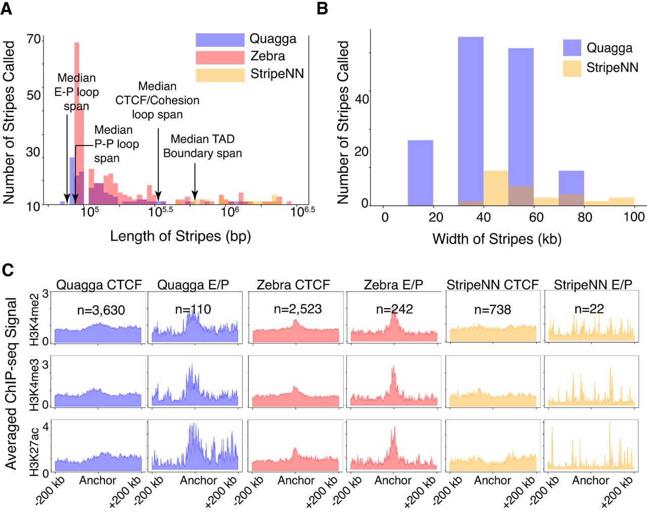
To assess EP-interacting stripes, we investigate the pileup of certain histone modifications around their main anchor position. Starting at the center of the width, we average the window of 200 kb upstream of and downstream from the anchor position across all stripes in the designated area. We examine H3K4me2 (strongly associated with promoters and enhancers), H3K4me3 (strong correlation to promoters), and H3K27ac (active enhancer mark) (Calo and Wysocka 2013). We compare CTCF-stripes to EP-stripes to emphasize the difference in signal. Enhancer/promoter activity forms very strong peaks in EP-stripes but is greatly diminished in CTCF-stripes in Quagga and Zebra (Fig. 5C). Stripenn shows H3K4me2/3 and H3K27ac are absent in CTCF-stripes, but those signals are also absent in its EP-stripes. It is reasonable that Stripenn's signals do not agree with EP-interaction behaviors as the lengths of its stripes trend very long, close to the behavior of TADs or long loops (300 kb to 1 Mb), so Stripenn's EP-stripes are most likely off-target and not EP interactions.

With accurate EP-stripes called by Quagga, we summarized the key characteristics of EP-stripes. First, the length is generally shorter than CTCF-stripes, which is near the median span of EP loops. Second, it is generally weaker than CTCF-stripes, as demonstrated by APA analysis (Supplemental Fig. 12), indicating an alternative mechanism for stripe formation. Just as with our comparison across tools, we observe the same EP-associated histone-tail modifications, showing cleaner peaks at 5 kb than at 10 kb (Supplemental Fig. 4C), whereas in our other experiments, Quagga is sensitive to a sequencing depth of as low as 125 million read pairs (Supplemental Fig. 3B).

Quagga is effective in Micro-C for H1-HESC EP-stripe detection

We investigate stripe detection on Hi-C and Micro-C for H1-hESCs (H1) to compare Quagga performance on the two data types and Quagga's ability to call classifiable stripes and minimize indeterminate stripes. Quagga run on H1 Hi-C calls 9677 stripes at P-value < 0.05: 90.9% CTCF-stripes, 3.97% EP-stripes, and 5.1% indeterminate (Fig. 6A). These percentages are consistent with our analysis of Quagga on GM12878 Hi-C. Quagga on H1 Micro-C calls 4192 stripes with more CTCF specificity and less indeterminate: 94.6% CTCF-stripes, 3.8% EP-stripes, and 1.6% indeterminate (Fig. 6B). Quagga run on either H1 or GM12878 still has a percentage of indeterminate stripe calls far below Zebra's (15.6%) or Stripenn's (12.9%). Quagga calls a much lower percentage of indeterminate stripes in Micro-C compared with Hi-C, which is related to better qualities of Micro-C data. Quagga's assigned stripe lengths fall within the expected median length for EP/PP interactions (41 and 71 kb, respectively), CTCF-loops (300 kb), and below median TAD spans (500 kb) (Fig. 6A,B). Quagga's stripe calls in H1-hESC Hi-C are nearly double those in H1 Micro-C, perhaps to differences in distance decay of contacts. For example, H1 Hi-C has 3.32 billion filtered read pairs with 51.0% being cis-long (>20 kb), but although H1-Micro-C similarly has 3.4 billion filtered read pairs, they are only 22.9% cis-long; these differences may affect the size of found stripes (Dekker et al. 2017).

Figure 6.

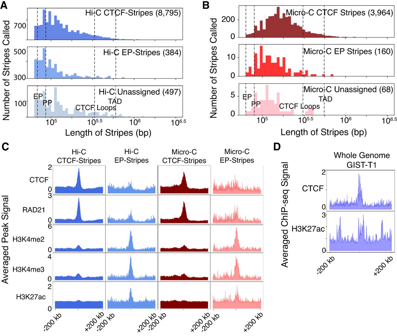
Comparing architectural stripes Quagga finds from Hi-C or Micro-C, their behavior is assessed as CTCF-stripes, EP-stripes, or as indeterminate stripes. (A) The distribution of stripe-lengths on Hi-C data falls into a majority around CTCF-stripe expected lengths. (B) Micro-C is similarly distributed, with less indeterminate stripes compared with indeterminate. (C) In an example stripe in H1-hESC Micro-C, no CTCF signal is present but H3K4me2 is present, suggesting this is an EP-stripe. (D) We show that global stripe detection on region capture Micro-C data recapitulates our observations in Hi-C and Micro-C for gastrointestinal stromal tumor (GIST-T1) cells.

Open in new tabDownload PowerPointLink to figure

Higher Hi-C stripe counts in H1 compared with GM12878 used in the comparison of tools are owing to differences in sequencing strategies; the Hi-C protocol for GM12878 used formaldehyde (FA) cross-linking and MboI digestion, whereas H1-hESC Hi-C was cross-linked with both FA and disuccinimidyl glutarate, digested with DpnII (Rao et al. 2014; Akgol Oksuz et al. 2021); the latter is a recent optimized sequencing protocol that resulted in better signal and loop recall, and it has been known that DpnII digestion is insensitive to CpG methylation when MboI is not (Belaghzal et al. 2017).

The difference in called stripe length and the number of stripes called is supported in the aggregate epigenomics pileup, in which we performed an epigenomic pileup of averaged transcription factor signal for CTCF-stripes or EP-stripes for Quagga stripe calls on Hi-C and Micro-C. CTCF-stripes were greatly enriched in CTCF and RAD21 in CTCF-stripes, whereas called EP-stripes were relatively dispersed or lacked well-defined CTCF or RAD21 peaks (Fig. 6C). For histone modifications characteristic to EP interactions, H3K4me2/3 and H3K27ac, these are more enriched in EP-stripe pileups than with the CTCF-stripes (Fig. 6C). Quagga H1 Hi-C peaks observed in isolating EP-stripes are recapitulated by the proportional percentage in Micro-C, and their epigenomic pileups match expectations for EP-stripe behavior: CTCF and RAD21 depleted, and H3K4me2, H3K4me3, and H3K27ac increased. This trend of enrichment is consistent with our expectation of depleting CTCF-anchored stripes (and, consequently, their loops) and also enriching a list of EP-stripes. Generally, the shorter stripes in H1 Hi-C tended to have clearer CTCF and RAD21 peaks, whereas H3K4me2/3 in H1 Micro-C appears to have marginally stronger epigenomic pileup peaks (Fig. 6C). Micro-C is known for a stronger distance decay factor and has a limited range for reliable signal beyond the main diagonal, so it is understandable that so many fewer CTCF-type stripes may be called. Despite the lower count, CTCF or EP classified stripes show a clear signal in their respective categories. Quagga was also able to find architectural stripes using region capture Micro-C data from gastrointestinal stromal tumor cells (Kim et al. 2024), in which we recapitulate the trend of CTCF and enhancer-related H3K27ac aggregation along the long axis anchor of the architectural stripes that Quagga calls there (Fig. 6D).

Quagga

Quagga is a chromatin stripe detection tool that works on 3C family sequencing types, particularly Hi-C and Micro-C, but Quagga also works with other contact frequency matrices, including HiChIP. Quagga uses image and signal processing techniques to do naive stripe calling and Poisson sampling over the length of stripes to determine stripe length and scores them with a P-value (Fig 1A). Quagga functions as a command-line application and a Python library, consisting of a main application, but makes its utilities and matrix operations available through the library's Quagga object. Users may take advantage of the included hg38, hg19, and mm9 or supply their own. Users may also specify their own parameters according to their needs in stripe detection, such as maximum distance off the main diagonal or how many cores to use. Additional information on installation and usage is documented at GitHub (https://github.com/dmcbffeng/StripeCaller/).

Input/output

Quagga requires an HIC or COOL file as well as a standard assembly file that matches the organism/version used to generate the Hi-C file. Quagga returns a BED-like file that specifies the chromosome, the coordinates of the stripe (its coordinates reflect the solved width), and the P-value determined. Users may specify a cutoff P-value for the ending stripes to be considered. Stripe integrity is already considered when forming the P-value, and the most full/intact stripe is output for any candidate; therefore, an integrity score is not necessary.

Quagga naive stripe calling

Statistical tests of stripe-like patterns

All stripes called are passed through a statistical test to determine if it is an artifact related to noise and to determine the starting and ending positions of the stripe relative to the main diagonal.

For example, to identify horizontal stripes, Quagga first calculates the observed contact value of each pixel on a candidate stripe and its neighbor regions. The observed value of the interaction between bins i and j (i¡j) is

Calculating stripe lengths

Because of sparsity or noise, the enrichment might not be significant for some pixels along the stripe. Therefore, after obtaining all P-values along the horizontal line, we allow breaking points when identifying stripes. The start and end positions are pinpointed as follows:

In the end, the significance (P-value) of the stripe is determined through the calculation

Minimizing computational cost

During Quagga's statistical tests, the slowest step is calculating the Poisson P-values. Because the significance of every pixel along the candidate stripe needs to be evaluated, Poisson P-values are calculated by (number of candidate stripes) × (maximum range for calculation)/(resolution) times, which is usually more than 1 million. We accelerate Quagga's calculation by storing all P-value calculation results in a self-balancing tree. Quagga only calculates P-values from scratch when the expected/observed values are already stored.

Let P(E, O) denote the P-value of Poisson statistics if the expected value is E and the observed value is O. Because the Poisson distribution is discrete, P(E_i, O_i) = P(E_i, floor(O_j)). Quagga stores all calculated floor(O_j) integer values. For each floor(O_j) value, it stores all calculated E_i in an AVL tree, which ensures the values are well sorted and can be queried and inserted at a short O(logN) time. When calculating P(E_j, O_j), Quagga searches the AVL tree with observed value = floor(O_j) and checks whether a similar expected value E_i was calculated before for this observed value. If an E_j with ${\displaystyle \frac{|E_j-E_j|}{E_i}<1\text{\%}}$ is found, we directly adapt the precalculated result of P(E_i, floor(O_j)) as P(E_j, floor(O_j)). In our benchmarking experiments, this approach accelerates Quagga's calculation by 100 times and only introduces <1% error in P-value estimation.

Data sets

To establish the performance of all the tools against one another and to determine the biological activity and validity of the computationally found stripes, we use many publicly available data sets. We list these in their entirety in Supplemental Tables 2 and 3; each following subsection will describe the cell line and data type in each case.

We build biological replicates of GM12878 Hi-C with data from 4DN Data Portal (https://data.4dnucleome.org/). To get a balanced sequencing depth of two replicates, we merge their technical replicates 1, 2, 3, 4, 5, and 11 of biological replicate 1 to obtain “biological replicate 1” in our study and merge their biological replicates 3, 4, and 5 to obtain “biological replicate 2” in our study. Both replicates have about 1100 million filtered reads.

Comparison of stripe calling methods and agreement of stripe calls

We explore the differences in tools and briefly calibrated stripe calls by choosing several regions of GM12878 hg38 Hi-C data and testing the ability of Quagga, Stripenn, Chromosight, and Zebra to find the hand-identified stripes, termed “diagnostic stripes.” The chromatin stripe caller, Zebra, is an implementation based on the original paper that programmatically identifies chromatin stripes, accessible via GitHub (https://github.com/XiaoTaoWang/StripeCaller). The tools Stripenn (Yoon et al. 2022) and Chromosight (Matthey-Doret et al. 2020) were used as is from their respective publications.

A reasonable set of parameters were established and run on GRCh38 (hg38) GM12878 Hi-C data set for all tools, and the recorded stripes were compared for the diagnostic stripe and exclusion of obvious false positives such as coordinates on the contact frequency matrix that neighbor zero-signal regions, as well as the start and end regions of a chromosome. By comparing the particular behaviors of each tool on the diagnostic stripes, as well as the off-target calls within those regions, an assessment of how each stripe caller is different can be made.

We used the default parameters for baseline methods, with only two modifications to avoid calling too many stripes: for Chromosight P = 0.3 and for Zebra fold-change = 1.4.

An interval intersection algorithm was written to detect consensus stripes between Zebra, Stripenn, Chromosight, and Quagga. Stripe coordinates of the base positions X1, X2 that are used in defining stripe width are used as the interval bounds. An intersection over the left (X1) or right (X2) bounds or the containment of either stripe by the other constituted detection as a matching, similar stripe. An allowance of ±2 kb was given to account for stripe caller error owing to biological noise. Matplotlib Venn diagram's package was used to visualize the resultant stripes, shown in Supplemental Figure 7.

APA of stripe lengths and widths and their distributions

To pile up the peaks to study stripe widths and their context sequences, we capture all 2 Mb windows around the main diagonal of the chromatin contact matrix that intersects with each stripe's major axis, averaging them for each tool: Zebra, Quagga, and Stripenn. Here, we still use GM12878 Hi-C data.

To study the relative integrity and distribution of lengths, we performed a size-scaling by lengths. For each stripe, we select the Hi-C region centered with width = 100 kb and length = 2× length called by the stripe caller and then zoom in/out to a fixed matrix size. For 3′ stripes, we rotate the region by 90° so that the stripe region can overlap with 5′ stripes in the pileup analysis.

The distributions for length and width of stripes were done, when possible, by determining the long and short “sides” of the rectangle each stripe caller solves, deeming the long side the length and the short side the width. Zebra may call multiple stripes along the same length, so we merged Zebra's many calls along a length when determining the 2 Mb APA window or other pileups to avoid multiple counting. All visualizations were done with Matplotlib.

CTCF and RAD21 enrichment analysis

ChIP-seq data of GM12878 CTCF and RAD21 are used to do ChIP-seq 1D pileup analysis. For the pileup analysis in Figure 3, A and B, we first select the stripe anchor and its ±1.5 Mb region (i.e., ±301 bins at 10 kb resolution) for each stripe and then count the average number of CTCF/RAD21 binding sites in each bin. We used CTCF binding motifs annotated by MotifMap to determine the orientation of CTCF binding. CTCF binding sites without CTCF motifs or with motifs in both orientations are removed in pileup analysis in Figure 3, C and D.

Stripe identity assignment

Based on the intersection of our stripe's narrow side (the stripe's width), we determine the stripe's identity as CTCF/cohesin-based stripes, EP interacting stripes, and indeterminate stripes. Intersections are found using a variation of a classical interval intersection algorithm, with a spacer to reflect inclusion or exclusion regions.

CTCF-stripes

To assign which stripes are CTCF/cohesin loop–based stripes, we intersect our stripes with JASPAR CTCF-motifs and check their occupancy state using GM12878 CTCF ChIP-seq peaks (Supplemental Table 2); stripes whose main axis anchor intersects with an occupied-CTCF motif were designated to be stripes composed of dynamic CTCF/cohesin loops, which we called CTCF-stripes. A spacer of ±50 kb along the coordinates along the stripe's width was included in the expanding intersection. Unoccupied CTCF motifs are not included for this assignment.

EP interacting stripes

Following previously established convention, we group all EP and PP activity together as EP interactions to describe EP-stripes. To determine EP interacting stripes (EP-stripes), we first determine what stripes have no CTCF motif or unoccupied-CTCF motifs (non-CTCF), which is found using a spacer exclusion-region of ±50 kb along the stripe's width. EP-stripes were determined by intersecting CTCF-deficient stripes with EP regions annotated by established 15-state ChromHMM annotations to identify enhancer/promoter regions (Ernst and Kellis 2012; Roadmap Epigenomics Consortium et al. 2015). We simplify the state annotation by combining all PP and EP activity (1:TssA, 2:TssAFlnk, 3:TxFlnk, 6:EnhG, 7:Enh, 11:BivFlnk, 12:EnhBiv), as other studies have, into an umbrella of “enhancer–promoter” interaction (Roadmap Epigenomics Consortium et al. 2015; Hsieh et al. 2022). Intersections of non-CTCF-stripes with EP annotations use an inclusive spacer of ±2 kb.

Indeterminate stripes

The subset of non-CTCF-stripes that are not assigned to enhancer promoter activity are deemed “indeterminate” stripes. These stripes intersect with neither occupied CTCF motifs nor ChromHMM state annotations linked with enhancer/promoter activity.

Epigenomic pileup analysis

As hundreds or thousands of stripes may be called, we sought to analyze our findings at a mass scale, so the aggregate epigenomic pileup analysis visualizes context sequence at and around called stripes to determine on-target/off-target calls. ChIP-seq for H3K4me1, H3K4me2, H3K27ac, CTCF, and RAD21 was used. For each pileup, we centered a window on the coordinate midpoint of the called stripe along its width. In the case of studying Hi-C and Micro-C, we used ±200 kb windows, averaging the resultant vector by stripe count. In the example Micro-C stripe, a window size of ±1.5 Mb was used; 500 nt bin ChIP-seq peaks were used in the pileups for all figures.

Comparison of H1-hESC Hi-C versus Micro-C stripes

We repeated our procedure used in GM12878 Hi-C for H1-hESC for Hi-C and Micro-C data sets. A similar strategy was used with H1-hESC CTCF motifs to determine CTCF-stripes and non-CTCF-stripes. We then used hg38 liftOver H1 ChromHMM annotations from another study, intersecting enhancer/promoter regions with stripes with no CTCF motifs or unoccupied CTCF motifs and designating these as likely EP-stripes (Ernst and Kellis 2012; Roadmap Epigenomics Consortium et al. 2015).

Code availability

The Quagga Python package is available at GitHub (https://github.com/dmcbffeng/StripeCaller) and as Supplemental Code. The code used to generate the figures in this manuscript is available at GitHub (https://github.com/seanpatrickmoran/Quagga_Analysis) and as Supplemental Code.

References

- ↵Akgol Oksuz B, Yang L, Abraham S, Venev SV, Krietenstein N, Parsi KM, Ozadam H, Oomen ME, Nand A, Mao H, 2021. Systematic evaluation of chromosome conformation capture assays. Nat Methods 18: 1046–1055. 10.1038/s41592-021-01248-7
- ↵Banigan EJ, van den Berg AA, Brandão HB, Marko JF, Mirny LA. 2020. Chromosome organization by one-sided and two-sided loop extrusion. eLife 9: e53558. 10.7554/eLife.53558
- ↵Barrington C, Georgopoulou D, Pezic D, Varsally W, Herrero J, Hadjur S. 2019. Enhancer accessibility and CTCF occupancy underlie asymmetric TAD architecture and cell type specific genome topology. Nat Commun 10: 2908. 10.1038/s41467-019-10725-9
- ↵Belaghzal H, Dekker J, Gibcus J. 2017. Hi-C 2.0: an optimized Hi-C procedure for high-resolution genome-wide mapping of chromosome conformation. Methods 123: 56–65. 10.1016/j.ymeth.2017.04.004
- ↵Calo E, Wysocka J. 2013. Modification of enhancer chromatin: what, how, and why? Mol Cell 49: 825–837. 10.1016/j.molcel.2013.01.038
- ↵Davidson IF, Bauer B, Goetz D, Tang W, Wutz G, Peters JM. 2019. DNA loop extrusion by human cohesin. Science 366: 1338–1345. 10.1126/science.aaz3418
- ↵Dekker J, Belmont AS, Guttman M, Leshyk VO, Lis JT, Lomvardas S, Mirny LA, O'Shea CC, Park PJ, Ren B, 2017. The 4D nucleome project. Nature 549: 219–226. 10.1038/nature23884
- ↵Dixon JR, Selvaraj S, Yue F, Kim A, Li Y, Shen Y, Hu M, Liu JS, Ren B. 2012. Topological domains in mammalian genomes identified by analysis of chromatin interactions. Nature 485: 376–380. 10.1038/nature11082
- ↵Ernst J, Kellis M. 2012. ChromHMM: automating chromatin-state discovery and characterization. Nat Methods 9: 215–216. 10.1038/nmeth.1906
- ↵Fudenberg G, Imakaev M, Lu C, Goloborodko A, Abdennur N, Mirny LA. 2016. Formation of chromosomal domains by loop extrusion. Cell Rep 15: 2038–2049. 10.1016/j.celrep.2016.04.085
- ↵Gabriele M, Brandão HB, Grosse-Holz S, Jha A, Dailey GM, Cattoglio C, Hsieh T-HS, Mirny L, Zechner C, Hansen AS. 2022. Dynamics of CTCF- and cohesin-mediated chromatin looping revealed by live-cell imaging. Science 376: 496–501. 10.1126/science.abn6583
- ↵Granlund GH. 1978. In search of a general picture processing operator. Comput Graph Image Process 8: 155–173. 10.1016/0146-664X(78)90047-3
- ↵Gupta K, Wang G, Zhang S, Gao X, Zheng R, Zhang Y, Meng Q, Zhang L, Cao Q, Chen K. 2022. StripeDiff: model-based algorithm for differential analysis of chromatin stripe. Sci Adv 8: eabk2246. 10.1126/sciadv.abk2246
- ↵Hsieh T-HS, Cattoglio C, Slobodyanyuk E, Hansen AS, Rando OJ, Tjian R, Darzacq X. 2020. Resolving the 3D landscape of transcription-linked mammalian chromatin folding. Mol Cell 78: 539–553.e8. 10.1016/j.molcel.2020.03.002
- ↵Hsieh T-HS, Cattoglio C, Slobodyanyuk E, Hansen AS, Darzacq X, Tjian R. 2022. Enhancer–promoter interactions and transcription are largely maintained upon acute loss of CTCF, cohesin, WAPL or YY1. Nat Genet 54: 1919–1932. 10.1038/s41588-022-01223-8
- ↵Kim KL, Rahme GJ, Goel VY, El Farran CA, Hansen AS, Bernstein BE. 2024. Dissection of a CTCF topological boundary uncovers principles of enhancer-oncogene regulation. Mol Cell 84: 1365–1376.e7. 10.1016/j.molcel.2024.02.007
- ↵Kraft K, Magg A, Heinrich V, Riemenschneider C, Schöpflin R, Markowski J, Ibrahim DM, Acuna-Hidalgo R, Despang A, Andrey G, 2019. Serial genomic inversions induce tissue-specific architectural stripes, gene misexpression and congenital malformations. Nat Cell Biol 21: 305–310. 10.1038/s41556-019-0273-x
- ↵Lieberman-Aiden E, van Berkum NL, Williams L, Imakaev M, Ragoczy T, Telling A, Amit I, Lajoie BR, Sabo PJ, Dorschner MO, 2009. Comprehensive mapping of long-range interactions reveals folding principles of the human genome. Science 326: 289–293. 10.1126/science.1181369
- ↵Matthey-Doret C, Baudry L, Breuer A, Montagne R, Guiglielmoni N, Scolari V, Jean E, Campeas A, Chanut PH, Oriol E, 2020. Computer vision for pattern detection in chromosome contact maps. Nat Commun 11: 5795. 10.1038/s41467-020-19562-7
- ↵Nora EP, Lajoie BR, Schulz EG, Giorgetti L, Okamoto I, Servant N, Piolot T, van Berkum NL, Meisig J, Sedat J, 2012. Spatial partitioning of the regulatory landscape of the X-inactivation centre. Nature 485: 381–385. 10.1038/nature11049
- ↵Rao SSP, Huntley MH, Durand N, Neva C, Stamenova EK, Bochkov ID, Robinson JT, Sanborn AL, Machol I, Omer AD, 2014. A 3D map of the human genome at kilobase resolution reveals principles of chromatin looping. Cell 59: 1665–1680. 10.1016/j.cell.2014.11.021
- ↵Roadmap Epigenomics Consortium, Kundaje A, Meuleman W, Ernst J, Bilenky M, Yen A, Heravi-Moussavi A, Kheradpour P, Zhang Z, Wang J, 2015. Integrative analysis of 111 reference human epigenomes. Nature 518: 317–330. 10.1038/nature14248
- ↵Sexton T, Yaffe E, Kenigsberg E, Bantignies F, Leblanc B, Hoichman M, Parrinello H, Tanay A, Cavalli G. 2012. Three-dimensional folding and functional organization principles of the Drosophila genome. Cell 148: 458–472. 10.1016/j.cell.2012.01.010
- ↵Vian L, Pękowska A, Rao SS, Kieffer-Kwon K-R, Jung S, Baranello L, Huang S-C, El Khattabi L, Dose M, Pruett N, 2018. The energetics and physiological impact of cohesin extrusion. Cell 173: 1165–1178.e20. 10.1016/j.cell.2018.03.072
- ↵Xi W, Beer MA. 2021. Loop competition and extrusion model predicts CTCF interaction specificity. Nat Commun 12: 1046. 10.1038/s41467-021-21368-0
- ↵Yoon S, Chandra A, Vahedi G. 2022. Stripenn detects architectural stripes from chromatin conformation data using computer vision. Nat Commun 13: 1602. 10.1038/s41467-022-29258-9
- ↵Zhang H, Emerson DJ, Gilgenast TG, Titus KR, Lan Y, Huang P, Zhang D, Wang H, Keller CA, Giardine B, 2019. Chromatin structure dynamics during the mitosis-to-G1 phase transition. Nature 576: 158–162. 10.1038/s41586-019-1778-y