
Abstract
The heterogeneity within, and similarities between, yeast chromosomes are studied. For the former, we show by the size distribution of domains, coding density, size distribution of open reading frames, spatial power spectra, and deviation from binomial distribution for C + G% in large moving windows that there is a strong deviation of the yeast sequences from random sequences. For the latter, not only do we graphically illustrate the similarity for the above mentioned statistics, but we also carry out a rigorous analysis of variance (ANOVA) test. The hypothesis that all yeast chromosomes are similar cannot be rejected by this test. We examine the two possible explanations of this interchromosomal uniformity: a common origin, such as genome-wide duplication (polyploidization), and a concerted evolutionary process.
The first completely sequenced genome of a eukaryotic organism, Saccharomyces cerevisiae (budding yeast) (Oliver et al. 1992; Dujon et al. 1994; Feldman et al. 1994; Johnston et al. 1994, 1997; Bussey et al. 1995, 1997; Murakami et al. 1995;Galibert et al. 1996; Bowman et al. 1997; Churcher et al. 1997;Dietrich et al. 1997; Jacq et al. 1997; Philippsen et al. 1997;Tettelin et al. 1997), provides a unique opportunity to analyze the compositional variations within and between chromosomes that form the genome. It has been known that there is a pervasive compositional heterogeneity in eukaryote DNA sequences (Macaya et. al. 1976; Bernardi 1989, 1995), that is, different regions of the same chromosome could be compositionally different. This heterogeneity is also manifested by the long-range statistical correlation in DNA sequences (Li et al. 1994; Li 1995–1998a, 1997a). When the correlation structure was measured more quantitatively, a surprising connection to a common form of long-ranged, multiple-scaled, slow-varying fluctuation in nature called “1/f noise” (e.g., see Li 1995–1998b) was discovered (Li 1992;Li and Kaneko 1992; Voss 1992).
Before the whole budding yeast genome was sequenced, it was rare to compare DNA sequences between different chromosomes owing to lack of data. Now this task is possible. At first glance, the 16 yeast chromosomes are quite different: The longest chromosome (chromosome IV with 1,531,974 bases) is 6.65 times the size of the shortest one (chromosome I with 230,209 bases), a considerable difference. A comparative display of C + G% from centromere to two telomeres for all chromosomes does not reveal any obvious common pattern. It has frequently been pointed out in the literature that the observation that yeast chromosome III has two C + G-rich peaks (Oliver et al. 1992;Sharp and Lloyd 1993), one for each arm, does not hold for other yeast chromosomes (Dujon 1996).
On the other hand, it was conjectured first by Smith (1987), then recently supported by a study by Wolfe and Shields (1997), that yeast may have experienced whole-chromosome duplication (polyploidization). If one chromosome was originally duplicated from another and if the subsequent evolutionary histories of the two were similar because of the shared cellular environment or if there are mechanisms to create and maintain the similarity between chromosomes, such as the reciprocal translocations (Sherman and Helms 1978; Sugawara and Szostak 1983;Breilmann et al. 1985; Ryu et al. 1996), the difference (in a statistical sense) between the two chromosomes should be small. The implication from this argument is that different chromosomes should share common features. We aim to resolve the two conflicting perspectives by studying both the intra- (within) and inter- (between) chromosomal heterogeneity in the yeast genome.
A commonly adopted procedure in presenting compositional variation along a chromosome is to plot C + G% in an overlapping moving window, (e.g., Oliver et al. 1992; Sharp and Lloyd 1993; Dujon 1996). However, features of this C + G% in the moving window plot can depend on both the window length and the moving distance. The total number of C + G-rich peaks may actually depend on how the window length and the moving distance are chosen. In this paper we use a unique set of nonoverlapping windows determined by a segmentation procedure, and the C + G% in these windows are tested using the analysis of variance (ANOVA) and similar rigorous treatments. We believe conclusions based on this method, concerning the statistical similarities and differences among the 16 chromosomes, are unambiguous.
RESULTS
Homogeneous Domains in Yeast Genome
Rather than treating a moving (overlapping) window with a fixed window size as a sample point of the C + G%, we use a systematic procedure to partition a sequence into (nonoverlapping) homogeneous domains. (This segmentation algorithm is described inBernaola-Galván et al. 1996; Román-Roldán et al. 1998; see Methods). There is a single parameter that controls how homogeneous a domain is: the significance level s. Whens is 99%, for example, there is a 99% chance that the segmentation is attributable to true heterogeneity and a 1% chance that such segmentation can be accomplished in a random sequence. The larger the s, the more stringent the criterion for the segmentation and the larger the domain size. For this reason,s can also be called the “stringency level.”
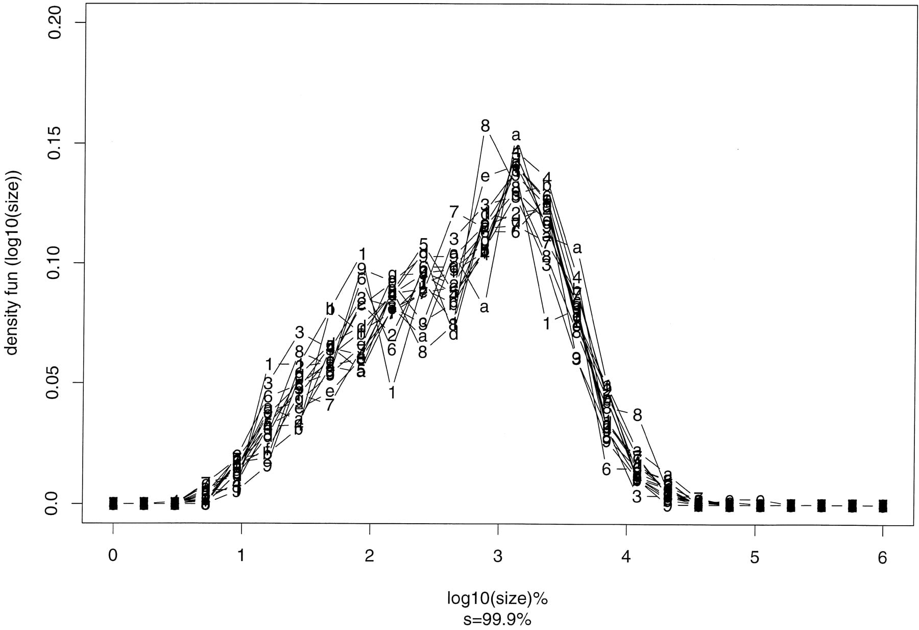
Table 1 lists the number of domains in all yeast chromosomes when the significance level s is 95%, 99%, 99.9%, 99.99%, and 99.999%. Each domain is relatively homogeneous at that significance level. At s = 95% and 99%, there are many domains with sizes smaller than 20 bases. Ats = 99.999%, the number of domains per chromosome is small, which is not ideal for carrying out statistical analysis. Thus, we choose s = 99.9%. Figure 1 shows the density function of the logarithm of domain sizes segmented at the significance level s = 99.9%. If no logarithm is taken, the distribution exhibits a long tail at large domain sizes.
Number of (Relative) Homogeneous Domains in All 16 Yeast Chromosomes Segmented at Different Significance (s) Levels
|
s
(%) | Chromosome no. | |||||||||||||||
| I | II | III | IV | V | VI | VII | VIII | IX | X | XI | XII | XIII | XIV | XV | XVI | |
| 95 | 1292 | 4663 | 1814 | 6377 | 3540 | 1670 | 6302 | 2984 | 2439 | 3502 | 3185 | 6132 | 5220 | 4436 | 6094 | 5404 |
| 99 | 448 | 1344 | 672 | 2765 | 1056 | 523 | 2017 | 975 | 732 | 1083 | 1140 | 1585 | 1684 | 1362 | 1923 | 1597 |
| 99.9 | 173 | 528 | 281 | 1068 | 398 | 203 | 707 | 349 | 379 | 404 | 481 | 729 | 678 | 433 | 754 | 708 |
| 99.99 | 105 | 295 | 147 | 587 | 227 | 103 | 421 | 189 | 218 | 207 | 285 | 367 | 355 | 393 | 242 | 384 |
| 99.999 | 78 | 194 | 96 | 388 | 120 | 70 | 211 | 121 | 122 | 124 | 204 | 257 | 195 | 193 | 7 | 204 |
Density function of logarithm of domain sizes (segmented at significance level s = 99.9%). The number of bins onx-axis is 25. Chromosomes I–IX are labeled 1–9; and chromosomes X–XVI are labeled a–g.
Testing Uniformity of C + G% between Different Chromosomes
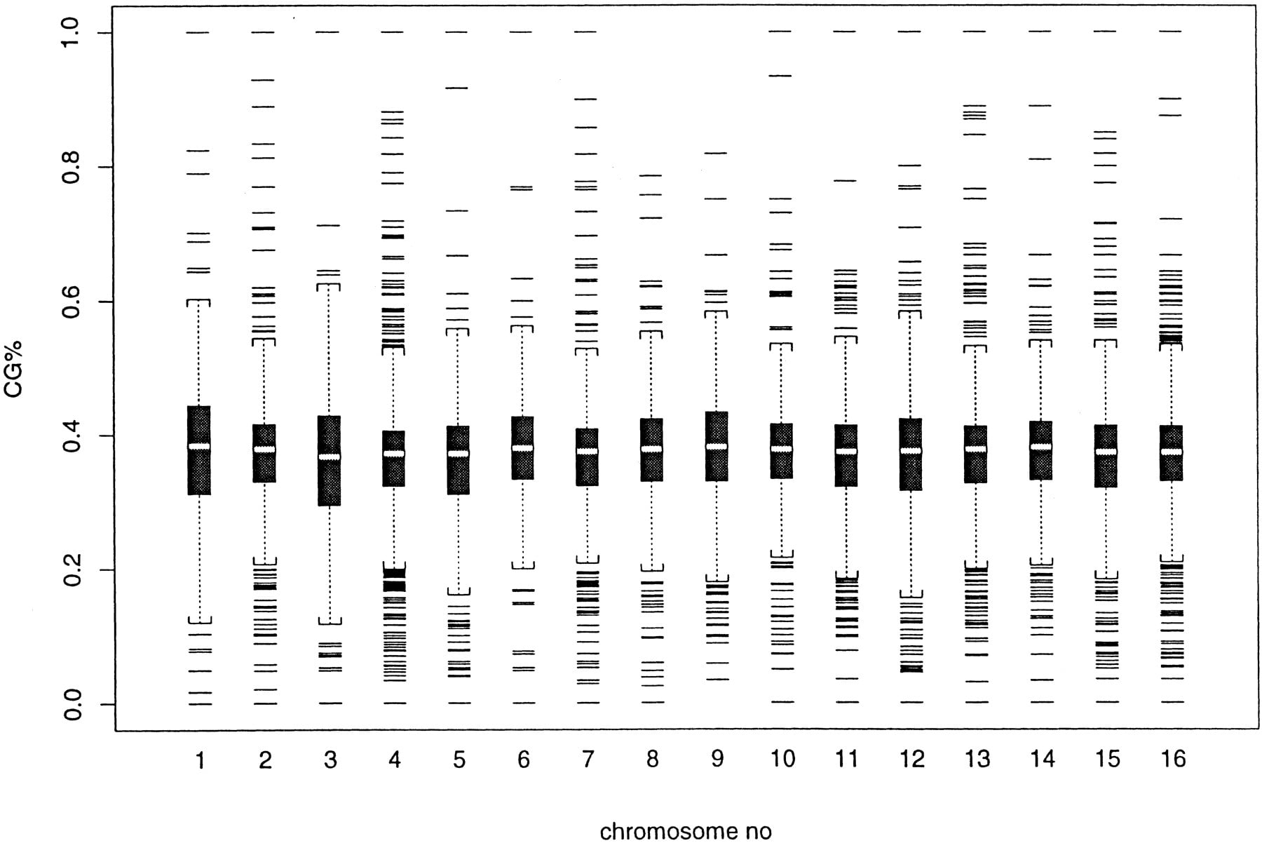
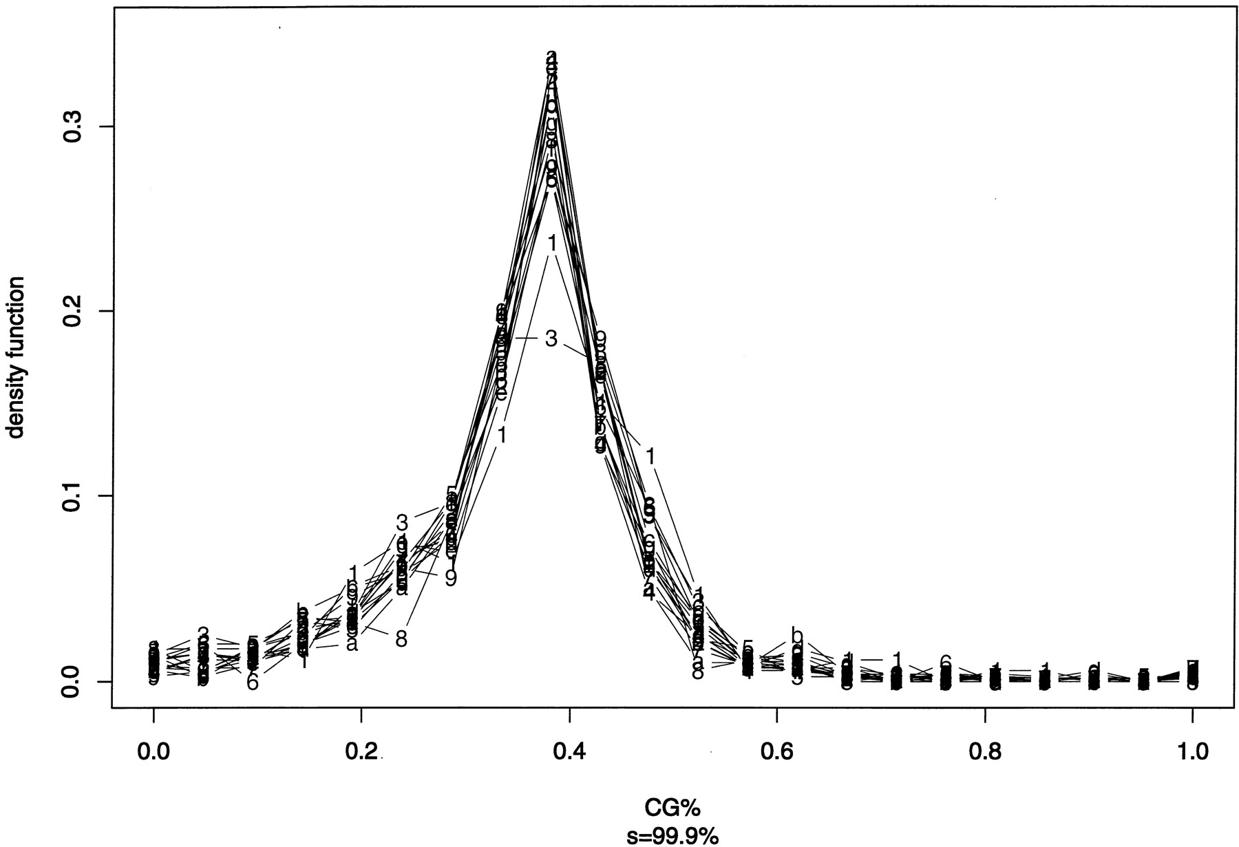
Despite the difference of domain sizes and the number of domains between 16 chromosomes, the similarity of the density function of (log) domain sizes in Figure 1 is obvious. Here, we examine the similarity of C + G% among different chromosomes. Using each domain segmented at the significance level of 99.9% as a sample point, we first show two exploratory plots: One is the box plot of C + G% (Fig.2), and the other is the density function of C + G% (Fig. 3). Because each domain contributes one sample point and domain sizes vary, the average or median presented in Figures 2 and 3 are not the same as the C + G% obtained from counting bases. In both Figure 2 and Figure3, chromosome I has the highest C + G%, and chromosome III is near the lowest end.
Box plot of C + G% in all 16 chromosomes, expressed as a fraction of 1. A box plot contains the following information: median (the middle line), first and third quartile (box), 1.5 of the interquartile distance (whisker), and outliers (top and bottom lines). This plot is obtained using the statistical package S-PLUS v. 3.4.
Density function of C + G% (expressed as a fraction of 1) in segmented domains (at significance level s = 99.9%). The bin size on x-axis is 0.0476 (=1/21). Chromosomes I–IX are labeled 1–9, and chromosomes X–XVI are labeleda–g.
ANOVA is a method to compare different groups (Fisher 1925, 1932). A test statistic, the F value, compares two quantities, one owing to the variance within group and the other owing to both the within- and between-group variances (see Methods). A large Fvalue means that one or more of the group means differs from the rest.
When the ANOVA is applied to yeast chromosomes, each chromosome is a group, and each segmented domain is a member of a group. Table2 shows the results of the ANOVA test at the significance level s = 99.9%. The F value in this test is equal to 1.037479, which is very small. With thisF value, the null hypothesis that all chromosomes have the same C + G% cannot be rejected (the probability that theF value will be this large or larger under the null hypothesis, i.e., the P value, is 0.4118962).
Analysis of Variance C + G% in Different Chromosomes
| SS | df | MS | F | Pvalue | |
| Among-chromosome | 0.1994 | 15 | 0.01329440 | 1.037479 | 0.4118962 |
| Within-chromosome | 105.8063 | 8257 | 0.01281413 |
[i] Each member is a C + G% of a domain segmented at the significance level s = 99.9%. (SS) Sum of squares of deviation; (df) degrees of freedom; (MS) mean square (i.e., SS/df); (F) the F-value ratio; (P value) the tail area under the distribution of F with the null hypothesis.
The derivation of the P value depends on an assumption that the C + G% follows a normal distribution. Because the distribution of C + G% as shown in Figure 3 does not look normal, we may not trust the P value obtained. A more robust test is the nonparametric Kruskal–Wallis test (Kruskal and Wallis 1952). Such a test was performed on the C + G% obtained ats = 99.9%, and it leads to a χ2 value of 21.3307 with 15 degrees of freedom, which corresponds to a p-value of 0.1266. Again, the null hypothesis cannot be rejected.
Similar ANOVA tests were carried out when the sequences are segmented at different significance levels. When s > 99.9%, the domains are larger, and F values are consistently small, thus failing to reject the null hypothesis. When s < 99%, there are many short “domains,” and their C + G% are very likely to be either 0 or 100%. Because domains of such small sizes are not of interest in terms of characterizing large-scale heterogeneity in DNA sequences, we prefer to choose a significance level ∼99.9% or larger.
Statistics of Open Reading Frames
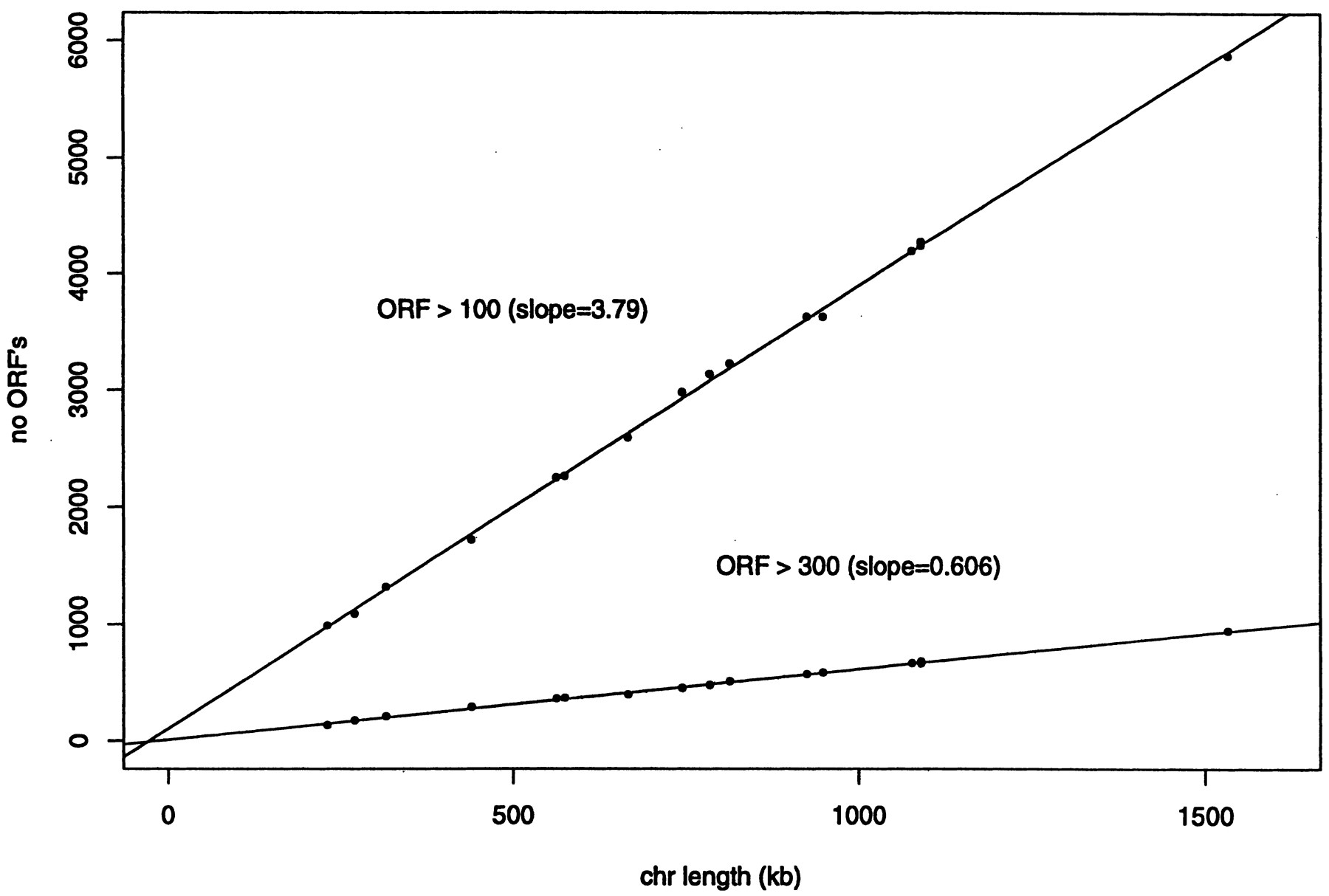
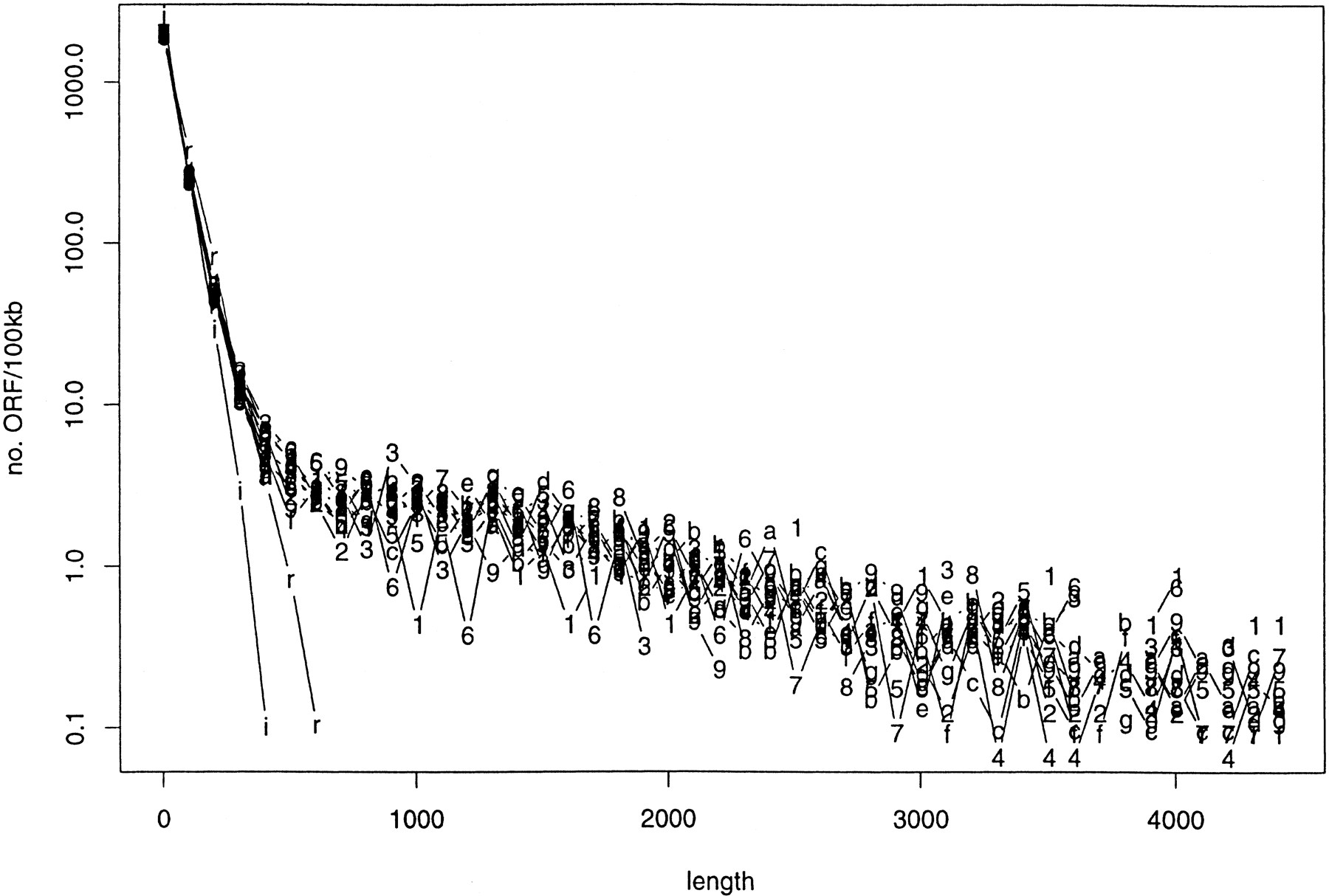
We define an open reading frame (ORF) as strictly a subsequence between a start and a stop codon, regardless of its length. When a start codon is followed by another start codon before encountering a stop codon, the first start codon is used. Figure 4shows the number of ORFs in each chromosome, when the size is >100 and 300 bases, as a function of the chromosome length. The linear increase in the number of ORFs with chromosome length indicates that the spatial density of ORF (i.e., coding density) is extremely uniform among different chromosomes.
Number of ORFs that are >100 and 300 bases, respectively, for each chromosome, as a function of the chromosome length. The regression lines have the slopes 3.7924 ± 0.0285 and 0.6058 ± 0.0067. The regression accounts for 99.9% and 99.8% of the variances, respectively, indicating an almost perfect modeling of the data with the linear function. The regression analysis is performed using the statistical package S-PLUS v. 3.4.
When the ORFs in one chromosome are examined, there are both long and short ones (remember that we define ORF without a reference to its length). As emphasized by Senapathy (1986), the length distribution of ORFs in a random sequence is negative exponential (or geometric). Consequently, if DNA sequences are random sequences, it would be very hard to observe long ORFs.
Figure 5 shows the length distribution (divided by the chromosome length, in the unit of 100 kb) of ORFs in all 16 yeast chromosomes (in linear-log scale). The corresponding distributions of ORFs of two random sequences are also illustrated for a comparison: one unbiased (ρ A = ρ C = ρ G = ρ T = 0.25) and another biased (ρ A = ρ T = 0.31 and ρ C = ρ G = 0.19, same base composition as the yeast chromosomes). Although there is a difference between unbiased and biased random sequences [C + G-poor random sequences tend to have shorter ORFs than unbiased ones (Oliver and Marín 1996), simply because stop codons are C + G-poor], the biggest difference is between a random sequence and a yeast sequence (Fig. 5).
Length distribution of ORFs (<4500) per 100 kb for all 16 chromosomes (labeled 1–9 and a–g), in linear-log scale. The similar distributions for two random sequences (r, unbiased; i, biased) are also plotted. The bin size on x-axis is 100 bases.
The similarity of length distribution of ORF’s among different chromosomes is striking. It is even more striking when we examine ORFs longer than 4500 bases—“outliers”—that are not included in Figure 5. The number of outliers per 100 kb is listed in Table3. With the exception of chromosome I (because there is only one outlier in that chromosome), the number of outliers per unit length is very similar among different chromosomes.
Number of Very Long ORFs (>4500 bases) per 100 kb for All 16 Yeast Chromosomes
| Chromosome no. | |||||||||||||||
| I | II | III | IV | V | VI | VII | VIII | IX | X | XI | XII | XIII | XIV | XV | XVI |
| 0.43 | 1.11 | 0.95 | 0.98 | 0.87 | 1.11 | 0.83 | 1.24 | 0.91 | 1.34 | 1.05 | 1.39 | 0.97 | 1.15 | 0.92 | 0.84 |
Spectral Analysis
A power spectrum is a transformation of a sequence of variables in the “frequency domain” or “frequency space.” There are at least two common applications of the spectral representation of a sequence. One is to examine whether or not the sequence is a random sequence that lacks correlation between different components: Random sequences exhibit flat power spectra. Sequences with flat power spectra are also known as “white noise.” Another application of the spectral representation is to identify underlying periodic patterns in the sequence: Each periodic signal is manifested as a peak in the power spectrum. For DNA sequences, the sequence of variables can either be the base sequence or can be the base density sequence where each base density is obtained from a nonoverlapping window (see Methods). The usefulness of spectral analysis for DNA sequences has well been recognized, such as the determination of the periodicity of ∼10 bases in genomic sequences (Widom 1996).
Figure 6 shows the 16 power spectra, one for each chromosome. Each chromosome is partitioned intoN = 214 = 16384 equal-length, nonoverlapping windows, and the base density in each window is used as the sequence for a spectral analysis. The inset in Figure 6, which is the regular power spectra multiplied by the chromosome length (in 100 kb), shows a remarkable similarity between the 16 chromosomes. There is a simple explanation of the multiplication of the sequence length: The base density is approximately equal to a constant plus a variance termO(1/√n), where n = L/N is the number of bases per window (L is the chromosome length). Inserting this expression in the definition of the power spectra (see Methods), the L dependence is 1/L. Multiplying by Lwill remove the L dependence.
Smoothed power spectra P(f) (in log–log scale) of density sequence for all 16 yeast chromosomes. The number of nonoverlapping windows is 214 = 16384. Neighboring 32 spectral components are averaged into one point. (Main plot) The original spectra; (inset) spectra multiplied by the chromosome length (in 100 kb).
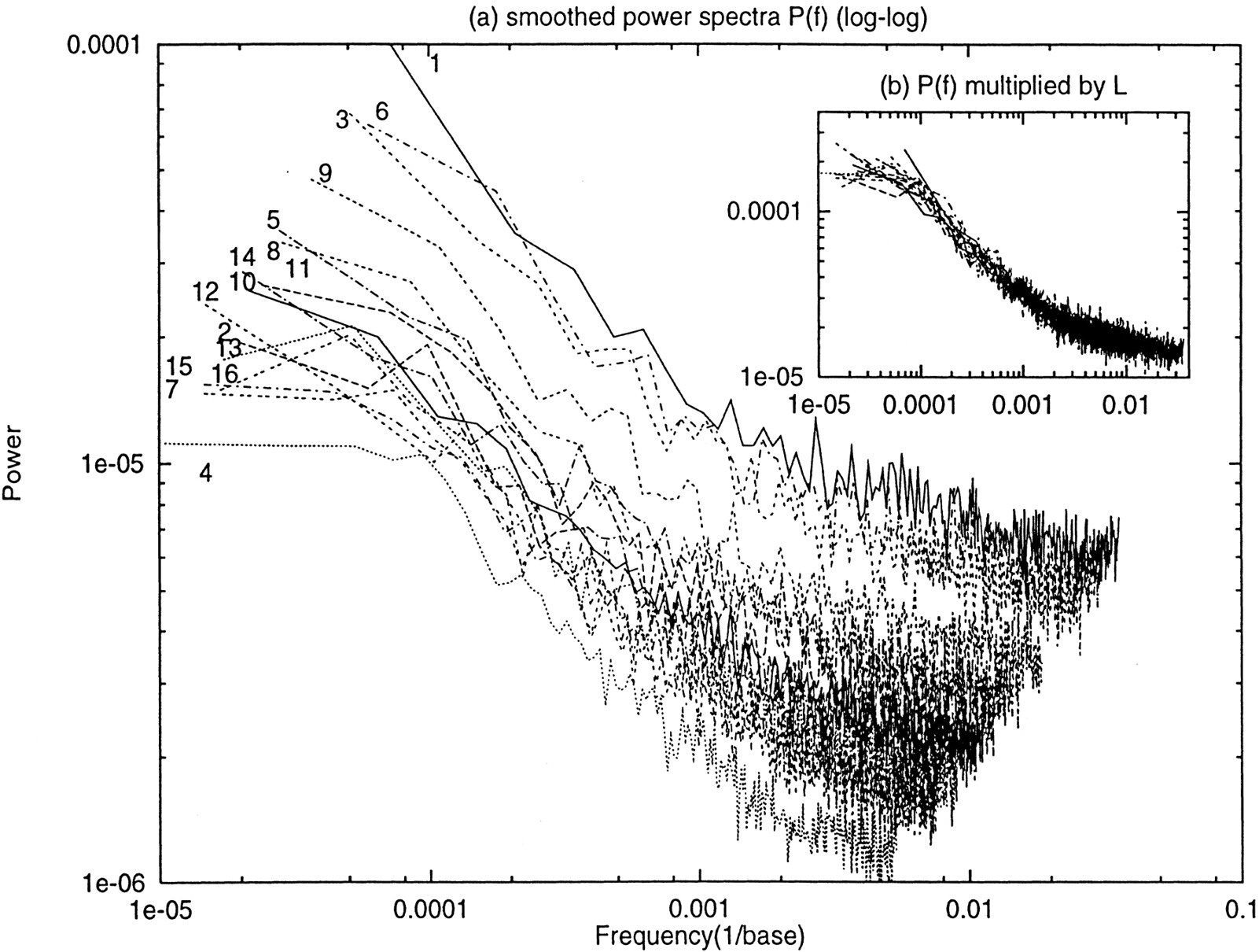
Another nontrivial observation of Figure 6 is that these are 1/f spectra. 1/f noise, also called “pink noise” (e.g., Dumermuth and Molinari 1987), is noise whose power spectra are approximately inversely proportional to the frequency. This form of noise is ubiquitous in nature, ranging from fluctuation of star luminosity to traffic flow density on highways (e.g., see Li 1995–1998b). 1/f noise is neither a white noise nor a 1/f 2 spectrum [the latter is typical for sequences with simple heterogeneity (Li 1997b)], and comparisons have been made among the three (Schroeder 1991). 1/f spectra are typical for sequences with a broad range of length scales, including long tails at the high end of the length scale. The presence of 1/f spectra in yeast chromosomes is consistent with the long tails in Figure 1 (remember that the logarithm compresses thex-axis at the high domain sizes) and Figure 5.
Overabundant Subsequences
A favorite analysis of DNA sequences is the frequency count of subsequences (“words”) in overlapping windows and comparing these with those from unbiased and biased random sequences. Instead of repeating this type of analysis, our aim here is to show that overabundancy of some subsequences is similar among yeast chromosomes.
We first show the overabundancy of subsequences of length 25. Because the number of possible subsequences with length 25 is 425 ≅ 1015, whereas the length of a yeast chromosome is ≤106 bases, most of the length 25 subsequences appear only once. We identify those length 25 subsequences that appear more than once in Figure 7, which plots the number of such subsequences for each chromosome. It is sometimes called a Zipf’s curve of the first kind (Miller 1965) (Zipf’s curve of the first type is often used for analyzing rare events, and Zipf’s curve of the second type for analyzing common events).
(Main plot) The histogram of the number of occurrences of length 25 subsequences, for all 16 yeast chromosomes (divided by the chromosome length). A similar histogram for the corresponding random sequence is also shown (i.e., every length 25 subsequences appear only once). (Inset) Marking the overabundant length 25 subsequences in chromosome VIII.
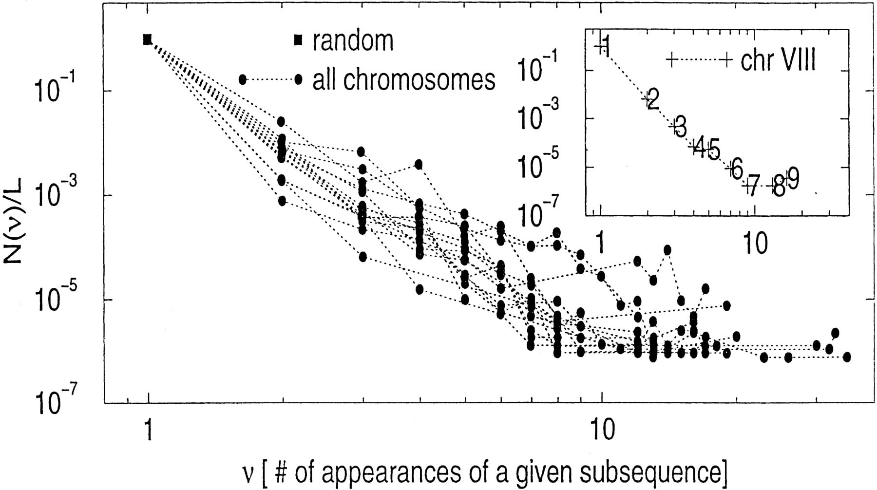
The inset in Figure 7 is the Zipf’s plot for chromosome VIII. We identify the most over-abundant length 25 subsequences in this chromosome as: ATAT…TA and TATA…AT[poly(AT) tract], (both appearing 16 times, no. 9),TT…T (appearing 13 times, no. 8) and AA…A(appearing 9 times, no. 7) [poly(A) and poly(T) tract], length 25 subsequences originated from a repeat element within the ORF YHR211W (part of nos. 6 and 5), and subsequences originated from aGTTTT repeat (part of nos. 5 and 4).
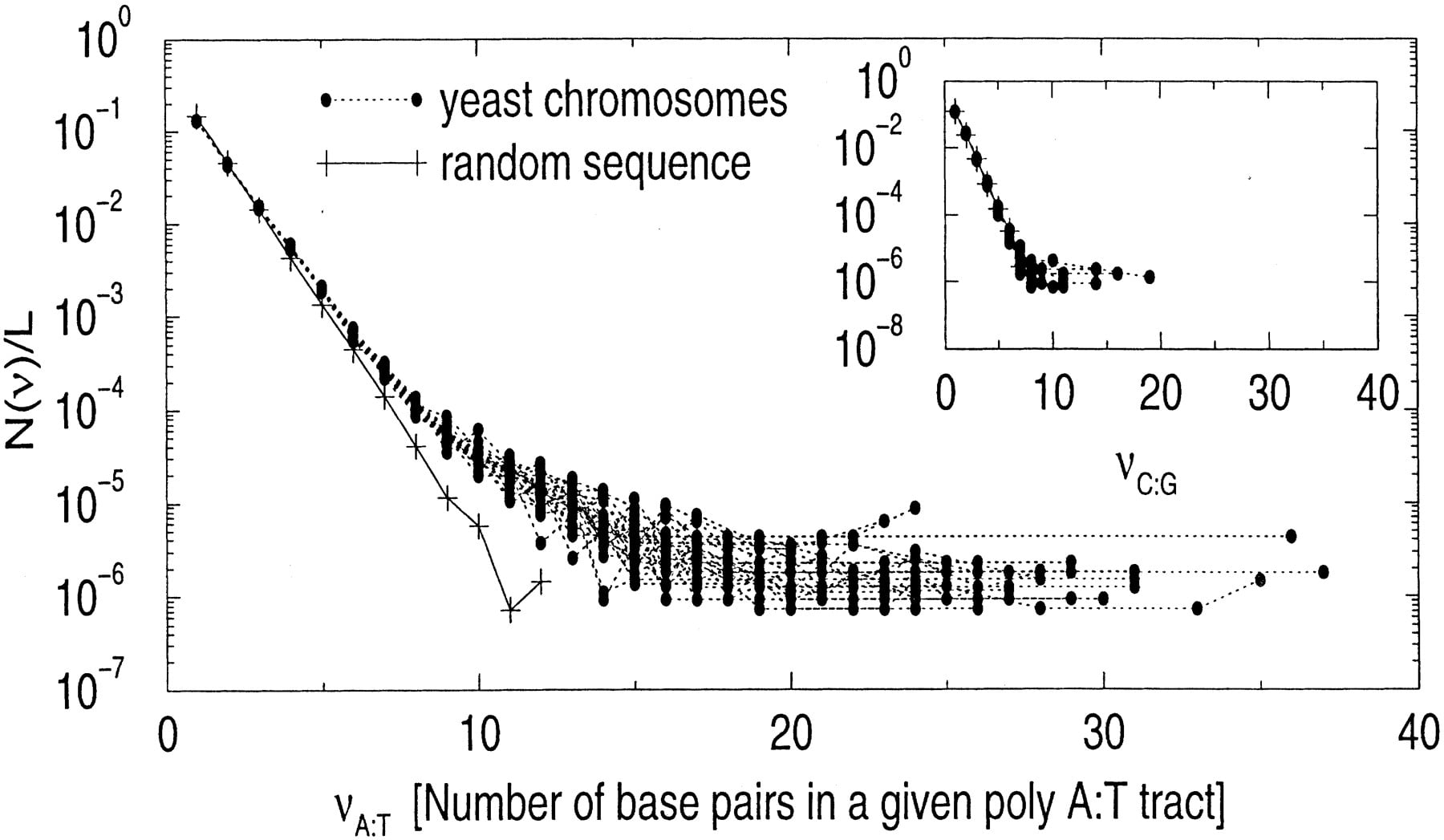
Poly(A)/poly(T) tracts are particularly abundant in yeast genome as part of poly-purine/poly-pyrimidine tracts (Yagil 1994; Behe 1995) We plot the length distribution of poly(A)/poly(T) tracts in Figure 8. In the inset in Figure 8, we plot the similar length distribution of poly(G)/poly(C) tracts, which is consistent with the corresponding random sequences. This indicates that poly-purine tracts are A-rich instead of G-rich.
(Main plot) The histogram (in linear-log scale) of the length of poly(A)/poly(T) tracts in all 16 yeast chromosomes (divided by chromosome length). A similar histogram for corresponding random sequences is also shown for a comparison (it is an exponential function). (Inset) Similar histogram for poly(C)/poly(G) tracts.
Again, what is striking about Figures 7 and 8 is that even rare events are qualitatively similar among different yeast chromosomes. We have already encountered this phenomenon in the frequency counts of very long ORFs (Table 3), which are also rare events.
Deviation from Binomial Distribution
The C + G% in overlapping windows (length n) in a random sequence follows the binomial distribution:
For yeast sequences, this distribution actually approximates the data well when the window size n is small (e.g., <30). For larger window sizes, however, the binomial distribution fails to fit the data, as can be seen from Figure 9. In Figure 9a, we plot this distribution for window size equal to 200 (for all 16 chromosomes).
(a) The histogram of C + G% for length 200 subsequences,P(Ncg,n ), for all 16 yeast chromosome sequences (in linearlog scale). (b) The second-order moment (variance) of the P(Ncg,n ) histogram as a function of the subsequence length n (in log–log scale). Two lines are also drawn for comparison: One is a linear function with slope equal to ρ cg (1 − ρ cg ); the other is a power-law function ∼n 1,5 (c) The third-order moment of the P(Ncg,n ) as a function ofn (in log–log scale). Two lines are also drawn for comparison: One is a linear function with slope equal to ρ cg (1 − ρ cg ) (1 − 2 ρ cg ); the other is a power-law function ∼n 3. d–f are similar toa–c for experimentally confirmed coding sequences.
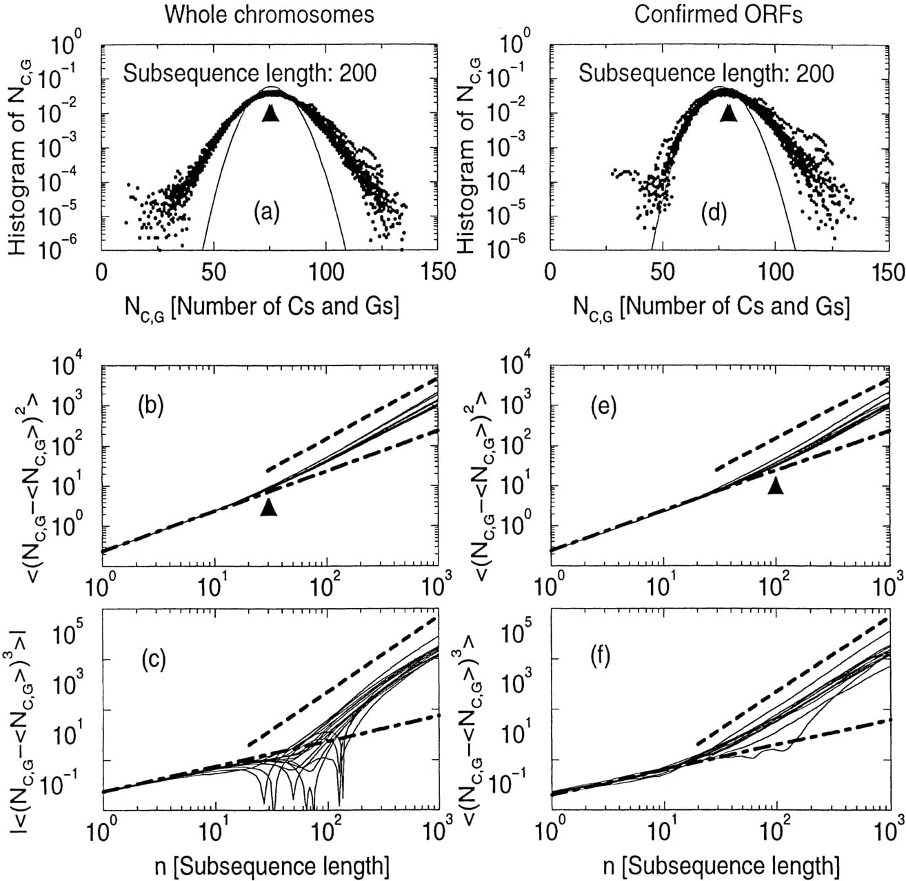
The wider spread in the distribution of Figure 9a can be characterized by the second-order moment (variance). Instead of plotting the similar distribution as Figure 9a for each window size n, in Figure 9b we plot the variance as the function of n from 1 to 1000 (again, for all 16 chromosomes). The binomial distribution predicts a linear increase of the variance on n with a slope ρ cg (1 − ρ cg ) (it is drawn in Fig. 9b). We can see that the deviation from the binomial distribution starts from ∼30 bases.
Another characterization of a distribution is its third-order moment, which measures the skewness of the distribution. Figure 9 plots this third-order moment (in absolute value) as a function of the window sizen. The binomial distribution predicts that this third-order moment increases linearly with n with the slope ‖ρ cg (1 − ρ cg )(1 − 2ρ cg )‖. Again, the deviation from the binomial distribution is clear when the window size is large.
We repeat similar plotting for experimentally confirmed coding sequences in Figure 9, d–f). The confirmed coding sequences are those ORFs whose locus description in the corresponding “Chromosomal Feature Table” of the Saccharomyces Genome Database (Cherry et al. 1997) is other than Hypothetical ORF. There is still a deviation from the binomial distribution, only with a lesser degree. The conclusion is the same: Even if each individual chromosome sequence exhibits deviations from a random sequence, this deviation is similar in different chromosomes.
DISCUSSION
Heterogeneity within Chromosomes
Our analysis of the primary DNA sequences in budding yeast reveals nonrandomness at large length scales, as illustrated by the long tail in the length distribution of homogeneous domains (Fig. 1), the existence of extremely long ORFs (Fig. 5), the 1/f-type power spectra (Fig. 6), and the deviation from the binomial distribution for long subsequences (Fig. 9). These features will not be revealed if one only examines short-range correlations such as the dinucleotide abundancy (Karlin and Mrázek 1997).
The degree of heterogeneity within a chromosome can be rigorously characterized and tested by what we called a “two-level segmentation test.” It should be noted that this test concerns the magnitude of the base composition fluctuation instead of spatial distances spanned by these fluctuations. The two-level segmentation test reveals that chromosomes III and VIII have larger fluctuation of C + G% than other chromosomes, even though the spatial structure of the fluctuation is similar among all chromosomes as shown in this paper. More details of this test will be presented elsewhere (J.L. Oliver and W. Li, in prep.)
Uniformity among 16 Chromosomes: Common Origin?
What we observe in this paper, that 16 yeast chromosomes are statistically similar to each other, may not be a surprise to many people. For example, Grantham proposed that the codon usage bias within a genome is similar, whereas those between different species are different (the so-called “genome hypothesis,” Grantham et al. 1980). A conclusion similar to ours was obtained (Lió et al. 1996) where block entropy is used to reveal compositional homogeneity at short length scales. What is new in this paper is a more systematic comparison of chromosome-wide statistics among different chromosomes. The ANOVA analysis and the related nonparametric test, in particular, provide a more quantitative characterization of C + G% difference or similarity between chromosomes.
Our results show with little doubt the uniformity among chromosomes. The question is, How can we explain it in light of the heterogeneity within a single chromosome? There could be two possible explanations: The first is that all 16 chromosomes might have originated from a limited set of ancestral chromosomes, either through repeated polyploidization, as occurred in many animal and plant genomes (Ohno 1970; Holland and Garcia-Fernández 1996; Spring 1997), or by a derivation from a single hypothetical ancestral chromosome through breakage and chromosomal rearrangements, as occurred in the genomes of cereals (Moore 1995; Moore et al. 1995).
A polyploid origin for the budding yeast genome was first proposed bySmith (1987) based on an evolutionary study of the histone genes. Recently, Wolfe and Shields (1997) reported evidence for an 8- to 16-chromosome doubling, though there is no stronger support for more ancestral duplications. Whether these ancient duplications occurred is still an open question. The extensive gene duplication present in the yeast genome would have profound implications for the evolution of new gene functions (Ohno 1970) and the correlation structure that this genome shows.
Uniformity among 16 Chromosomes: Concerted Evolution?
The second explanation is that whether or not all chromosomes originated from the same source, they could evolve together either “passively” or “actively.” By passively, we mean these chromosomes were expressed, replicated, and repaired in the same cellular environment. By actively, we mean some mechanism that forces different chromosomes to have similar sequences.
Although repetitive sequences could be such a forcing mechanism—the similar repetitions in all chromosomes may cause these chromosomes to be statistically similar—it is known that the yeast genome is remarkably poor in tandem repetitive sequences (Dujon 1996) [the best known repetitive sequences in yeast, the subtelomeric repeats (Szostak and Blackburn 1982; Chan and Tye 1983a,b), are only located near the two ends of the chromosome]. Also, repetitive sequences are not the most important contributor to the nonrandomness of a DNA sequence. They can be easily separated from the rest of the sequence, and the remainder of the sequence will still exhibit compositional heterogeneity and statistical correlation (Li 1992).
The insertion of mobile elements such as transposons in yeast (Ty) (Boeke and Sandmeyer 1991), which are bracketed by long-terminal repeats (LTRs), can possibly contribute to the uniformity because they introduce similar segments into different chromosomes. However, Ty and LTRs constitute only 3.15% of the yeast genome (Dujon 1996). Furthermore, yeast transposon seems to insert in specific regions, and its density is very different from one chromosome to another; thus, it is unlikely that it is primarily responsible for the pervasive interchromosome uniformity we observed.
One of the best candidates for forcing uniformity among different yeast chromosomes is the interchromosome recombination (e.g., through reciprocal translocation), despite the higher meiotic cost related to this interchange (Sherman and Helms 1978; Sugawara and Szostak 1983;Breilmann et al. 1985; Ryu et al. 1996). This mechanism is supported by the observation that most of the duplicated gene clusters maintain the same orientation toward the centromere (Wolfe and Shields 1997). Recombinant events, such as reciprocal translocation, ensure a recurrent interchromosome genetic flux, which may lead to uniformity among different chromosomes.
If reshuffling chromosomal segments forces uniformity among different chromosomes, why did the same mechanism not force homogeneity within a chromosome? One possibility is that although interchromosome recombinations are common (Sherman and Helms 1978; Sugawara and Szostak 1983; Breilmann et al. 1985; Ryu et al. 1996), the internal rearrangements within a same chromosome (through inversion) are less frequent. It is also possible that the interchromosome recombinations act only on a large length scale; thus, all nonrandomness in smaller scales is untouched. A definite answer to this question requires further investigation.
The molecular and evolutionary knowledge obtained from the yeast genome provides essential clues to understanding the general problem of complex heterogeneity in eukaryotic DNA sequences. Current models of genome dynamics consider single-base duplication and point mutation (Li 1989, 1991), nonlocal duplication (Li 1992), and insertion of mobile elements (Buldyrev et al. 1993). Despite their extreme simplicity, some of these models, such as the expansion-modification model (Li 1989,1991), are able to generate complex heterogeneity, self-similar long-range correlation, and 1/f power spectra. None of them, however, considers multiple chromosome dynamics, such as the whole-genome duplication and interchromosomal exchange mentioned above. It is conceivable that by adding these genome-wide dynamics to the single-sequence models, both intrachromosome heterogeneity and interchromosome uniformity can be simulated and explained.
METHODS
Segmentation Algorithm
A DNA sequence is segmented into (relatively) homogeneous domains by the following 1-to-2 and recursive 1-to-2 segmentation algorithm (Bernaola-Galván et al. 1996; Román-Roldán et al. 1998): In the 1-to-2 segmentation, for each partition point i(1 ≤ i ≤ L − 1, where L is the sequence length), the Jensen-Shannon distance (Lin 1991) between the left and right subsequences, D(i), is calculated:
In recursive 1-to-2 segmentation, the above 1-to-2 segmentation is recursively applied to each segmented domain until (1) the size of the domain is equal to 1 base (or smaller than a selected lower bound) or (2) the D(i*) falls within the s% of the distribution under null hypothesis (i.e., the sequence is a random sequence). The s is called the significance level in this paper (note that in many statistics books, 1 − s is called the significance level), which is usually chosen to be high (stringent), for example, 99% or 99.9%. A computer program for segmenting DNA sequences is available upon request (J.L. Oliver, R. Román-Roldán, J. Alegre, J. Pérez, P. Bernaola-Galván, in prep.).
ANOVA
The single-classification ANOVA is introduced in great detail bySokal and Rohlf (1995). Denoting the jth member inith group as Yij, and the average ofYij over j as Y i ,the average of Y i over i as Y ,the following within- and between-sum of squares (SS) are calculated: SS w = Σ i Σ j (Yij − Y i )2, SS a = Σ i ni ( Y i − Y )2, where ni is the number of members in groupi. If the number of groups is a, the within-, and between-degrees of freedom are given by df w = Σ i (ni − 1), df a = a − 1. The sum of the squares divided by the degree of freedom is called the mean of squares (MS), and the ratio of the two MSs is the F value:
Power Spectra
A power spectrum can be defined for a base sequence or a density sequence. When it is defined for a base sequence of DNA, it is
To take advantage of the fast Fourier transform algorithm (Cooley and Tukey 1965), the number of data points to be analyzed should be a power of 2, that is, N = 2m, where m is an integer.
P(k)s are often plotted as a function of the frequency f = k/L, which ranges from 0 to 0.5 in the unit of 1/base. We smooth a noisy plot ofP(k) by averaging neighboring spectral components (Press et al. 1990).
W.L.’s work is supported by grant K01HG00024 from the National Institutes of Health (NIH). Part of the results were presented at the “Identifying Features in Biological Sequences Workshop” (Aspen, CO; June 1996). Partial support from the workshop to W.L. and partial support from grant HG00008 (NIH, to J. Ott) is acknowledged. G.S. acknowledges support from the Mathers Foundation to the Center for Physics and Biology at Rockefeller University. J.L.O. and P.B.G.’s work is supported by grants PB96-1414-CO2-01 from the Spanish Government. We thank Andrés Aguilera, Oliver Clay, Albert Libchaber, Antonio Marin, Manuel Ruíz-Rejón, and Federico Stefanini for comments and Katherine Montague for proofreading the draft.
The publication costs of this article were defrayed in part by payment of page charges. This article must therefore be hereby marked “advertisement” in accordance with 18 USC section 1734 solely to indicate this fact.
Notes
[2] Present address: IBM T.J. Watson Research Center, Yorktown Heights, New York 10598 USA.
[3] Corresponding author.
Notes
[4] E-MAIL [email protected]; FAX (212) 327-7996.
REFERENCES
- ↵M.J. Behe(1995) An overabundance of long oligopurine tracts occurs in the genome of simple and complex eukaryotes. Nucleic Acids Res. 23:689–695.
- ↵P. Bernaola-GalvánR. Román-RoldánJ.L. Oliver(1996) Compositional segmentation and long-range fractal correlations in DNA sequences. Phys. Rev. E 53:5181–5189.
- ↵G. Bernardi(1989) The isochore organization of the human genome. Annu. Rev. Genetics 23:637–661.
- ↵(1995) The human genome: Organization and evolutionary history. Annu. Rev. Genetics 29:445–476, ibid.
- ↵J.D. BoekeS.B. Sandmeyer(1991) Yeast transposable elements. in The molecular and cellular biology of the yeast Saccharomyces: Vol. I. Genome dynamics, protein synthesis, and energetics, eds J.R. BroachJ.R. PringleE.W. Jones(Cold Spring Harbor Laboratory Press, Cold Spring Harbor, NY), pp 193–261.
- ↵S. BowmanC. ChurcherK. BadcockD. BrownT. ChillingworthR. ConnorK. DedmanS. GentlesN. HamlinS. Hunt(1997) The nucleotide sequence of Saccharomyces cerevisiae chromosome XIII. Nature (Suppl.) 387:90–93.
- ↵D. BreilmannJ. GafnerM. Ciriacy(1985) Gene conversion and reciprocal exchange in a Ty-mediated translocation in yeast. Curr. Genet. 9:553–560.
- ↵S.V. BuldyrevA.L. GoldbergeS. HavlinC.K. PengH.E. StanleyM.H.R. StanleyM. Simons(1993) Fractal landscapes and molecular evolution: Modeling the Myosin heavy chain gene family. Biophys. J. 65:2673–2679.
- ↵H. BusseyD.B. KabackW. ZhongD.T. VoM.W. CloakN. FortinJ. HallB.F. OuelletteT. KengA.B. Barton(1995) The nucleotide sequence of chromosome I from Saccharomyces cerevisiae. Proc. Natl. Acad. Sci. 92:3809–3813.
- ↵H. BusseyR.K. StormsA. AhmedK. AlbermannE. AllenW. AnsorgeR. AraujoA. AparicioB. BarrellK. Badcock(1997) The nucleotide sequence of Saccharomyces cerevisiae chromosome XVI. Nature (Suppl.) 387:103–105.
- ↵C.S.M. ChanB.K. Tye(1983a) Organization of DNA sequences and replication origins at yeast telomeres. Cell 33:563–573.
- ↵(1983b) A family of Saccharomyces cerevisiae repetitive autonomously replicating sequences that have very similar genomic environments. J. Mol. Biol. 168:505–523, ibid.
- ↵J.M. CherryC. BallS. ChervitzS. DwightM. HarrisE. HesterG. JuvikA. MalekianT. RoeS. WengD. Botstein(1997) Saccharomyces Genome Database. http://genome-www.stanford.edu/Saccharomyces/.
- ↵C. ChurcherS. BowmanK. BadcockA. BankierD. BrownT. ChillingworthR. ConnorK. DevlinS. GentlesN. Hamlyn(1997) The nucleotide sequence of Saccharomyces cerevisiae chromosome IX. Nature (Suppl.) 387:84–87.
- ↵J.W. CooleyJ.W. Tukey(1965) An algorithm for machine computation of complex Fourier series. Math. Computation 19:297–301.
- ↵F.S. DietrichJ. MulliganK. HennessyM.A. YeltonE. AllenR. AraujoE. AvilesA. BernoT. BrennanJ. Carpenter(1997) The nucleotide sequence of Saccharomyces cerevisiae chromosome V. Nature (Suppl.) 387:78–81.
- ↵B. Dujon(1996) The yeast genome project: What did we learn? Trends Genet. 12:263–270.
- ↵B. DujonD. AlexandrakiB. AndreW. AnsorgeV. BaladronJ.P.G. BallestaA. BanreviP.A. BolleM. Bolotin-FukuharaP. Bossier(1994) Complete DNA sequence of yeast chromosome XI. Nature 369:371–378.
- B. DujonK. AlbermannM. AldeaD. AlexandrakiW. AnsorgeJ. ArinoV. BenesC. BohnM. Bolotin-FukuharaR. Bordonné(1997) The nucleotide sequence of Saccharomyces cerevisiae chromosome XV. Nature (Suppl.) 387:98–102.
- ↵G. DumermuthL. Molinari(1987) in Methods of analysis of brain electrical and magnetic signals, eds A.S. GevinsA. Remond(Elsevier, Amsterdam, The Netherlands), pp 85–130.
- ↵H. Feldmann(1994) Complete DNA sequence of yeast chromosome II. EMBO J. 13:5793–5809.
- ↵R.A. Fisher(1925) Statistical methods for research workers (Oliver & Boyd, Edinburgh, UK), 1st ed..
- ↵(1932) The design of experiments. (Oliver & Boyd, Edinburgh, UK) ibid.
- ↵F. GalibertD. AlexandrakiA. BaurE. BolesN. ChalwatzisJ.-C. ChuatF. CosterC. CziepluchM. De HaanH. Domde(1996) Complete nucleotide sequence of Saccharomyces cerevisiae chromosome X. EMBO J. 15:2031–2049.
- ↵E. GranthamC. GautierM. GouyR. MercierA. Pavé(1980) Codon catalog usage and the genome hypothesis. Nucleic Acids Res. 8:r49–r62.
- ↵P.W. HollandJ. Garcia-Fernández(1996) Hox genes and chordate evolution. Dev. Biol. 173:382–395.
- ↵C. JacqJ. Alt-MórbeB. AndreW. ArnoldA. BahrJ.P.G. BallestaM. BarguesL. BaronA. BeckerN. Biteau(1997) The nucleotide sequence of Saccharomyces cerevisiae chromosome IV. Nature (Suppl.) 387:75–78.
- ↵M. JohnstonS. AndrewsR. BrinkmanJ. CooperH. DingJ. DoverZ. DuA. FavelloL. FultonS. Gattung(1994) Complete nucleotide sequence of Saccharomyces cerevisiae chromosome VIII. Science 265:2077–2082.
- ↵M. JohnstonL. HillierL. Rilesother members of the Genome Sequencing CenterK. AlbermannB. AndreW. AnsorgeV. BenesM. BrücknerH. Delius(1997) The nucleotide sequence of Saccharomyces cerevisiae chromosome XII. Nature (Suppl.) 387:87–90.
- ↵S. KarlinJ. Mrázek(1997) Compositional differences within and between eukaryotic genomes. Proc. Natl. Acad. Sci. 94:10227–10232.
- ↵W.H. KruskalW.A. Wallis(1952) Use of ranks in one-criterion variance analysis. J. Am. Stat. Assoc. 47:583–621.
- ↵W. Li(1989) Spatial 1/f spectra in open dynamical systems. Europhys. Letts. 10:395–400.
- ↵(1991) Expansion-modification systems: A model for spatial 1/f spectra. Phys. Rev. A 43:5240–5260, ibid.
- ↵(1992) Generating non-trivial long-range correlations and 1/f spectra by replication and mutation. Int. J. Bifurcation Chaos. 2:137–154, ibid.
- Li, W., ed. 1995–1998a. A bibliography on studies of correlation structures of DNA sequences. http://linkage.rockefeller.edu/wli/dna_corr/.
- Li, W., ed. 1995–1998b. A bibliography on 1/f noise. http://linkage.rockefeller.edu/wli/1fnoise/.
- (1997a) The study of correlation structure of DNA sequences—A critical review. Comput. & Chem. 21:257–272, ibid.
- (1997b) The complexity of DNA: The measure of compositional heterogeneity in DNA sequences and measures of complexity. Complexity 3:33–37, ibid.
- ↵W. LiK. Kaneko(1992) Long-range correlation and partial 1/f spectrum in a non-coding DNA sequence. Europhys. Letts. 17:655–660.
- ↵W. LiT.G. MarrK. Kaneko(1994) Understanding long-range correlations in DNA sequences. Phys. D 75:392–416, [erratum 82: 217]..
- ↵J. Lin(1991) Divergence measures based on the Shannon entropy. IEEE Trans. Inf. Theory 37:145–151.
- ↵P. LióA. PolitiM. BuiattiS. Ruffo(1996) High statistics block entropy measures of DNA sequences. J. Theoret. Biol. 180:151–160.
- ↵G. MacayaJ.P. ThieryG. Bernardi(1976) An approach to the organization of eukaryotic genomes at a macromolecular level. J. Mol. Biol. 108:237–254.
- ↵G.A. Miller(1965) “Preface” of Psycho-biology of languages by G.K. Zipf. (MIT Press, Cambridge, MA).
- ↵G. Moore(1995) Cereal genome evolution: Pastoral pursuits with ’Lego’ genomes. Curr. Opin. Genet. Dev. 5:717–724.
- ↵G. MooreT. FooteT. HelentjarisK. DevosN. KurataN. Gale(1995) Was there a single ancestral cereal chromosome? Trends Genet. 11:81–82.
- ↵Y. MurakamiM. NaitouH. HagiwaraT. ShibataM. OzawaS.I. SasanumaM. SasanumaY. TsuchiyaE. SoedaK. Yokoyama(1995) Analysis of the nucleotide sequence of chromosome VI from Saccharomyces cerevisiae. Nature Genet. 10:261–268.
- ↵S. Ohno(1970) Evolution by gene duplication. (Springer-Verlag, Berlin, Germany).
- ↵J.L. OliverA. Marín(1996) A relationship between GC content and coding-sequence length. J. Mol. Evol. 43:216–223.
- ↵S.G. OliverQ.J.M. van der AartM.L. Agostoni-CarboneM. AigleL. AlberghinaD. AlexandrakiG. AntoineR. AnwarJ.P.G. BallestaP. Benit(1992) The complete DNA sequence of yeast chromosome III. Nature 357:38–46.
- ↵P. PhilippsenK. KleineR. PöhlmannA. DüsterhöftK. HambergJ.H. HegemannB. ObermaierL.A. UrrestarazuR. AertK. Albermann(1997) The nucleotide sequence of Saccharomyces cerevisiae chromosome XIV and its evolutionary implications. Nature (Suppl.) 387:93–98.
- ↵W.H. PressS.A. TeukolskyW.T. VetterlingB.P. Flannery(1990) Numerical recipes in C. (Cambridge University Press, Cambridge, UK).
- ↵R. Román-RoldánP. Bernaola-GalvánJ.L. Oliver(1998) Sequence compositional complexity of DNA through an entropic segmentation algorithm. Phys. Rev. Letts. 80:1344–1347.
- ↵S.L. RyuY. MurookaY. Kaneko(1996) Genomic reorganization between two sibling yeast species Saccharomyces bayanus and Saccharomyces cerevisiae. Yeast 12:757–764.
- ↵M. Schroeder(1991) Fractals, chaos, power laws. (W.H. Freeman & Co. New York, NY).
- ↵P. Senapathy(1986) Origin of eukaryotic introns: A hypothesis, based on codon distribution statistics in genes, and its implications. Proc. Natl. Acad. Sci. 83:2133–2137.
- ↵P.M. SharpA.T. Lloyd(1993) Regional base composition variation along yeast chromosome III: Evolution of chromosome primary structure. Nucl. Acids Res. 21:179–183.
- ↵F. ShermanC. Helms(1978) A chromosomal translocation causing overproduction of iso-2-cytochrome c in yeast. Genetics 88:689–707.
- ↵M.M. Smith(1987) Molecular evolution of the Saccharomyces cerevisiae histone gene loci. J. Mol. Evol. 24:252–259.
- ↵R.R. SokalF.J. Rohlf(1995) Biometry (W.H. Freedman & Co. New York, NY), 3rd ed..
- ↵J. Spring(1997) Vertebrate evolution by interspecific hybridisation—Are we polyploid? FEBS Lett. 400:2–8.
- ↵N. SugawaraJ.W. Szostak(1983) Recombination between sequences in nonhomologous positions. Proc. Natl. Acad. Sci. 80:5675–5679.
- ↵J.W. SzostakE.H. Blackburn(1982) Cloning yeast telomeres on linear plasmid vectors. Cell 29:245–255.
- ↵H. TettelinM.L. Agostoni-CarboneK. AlbermannM. AlbersJ. ArroyoU. BackesT. BarreirosI. BertaniA.J. BjoursonM. Brückner(1997) The nucleotide sequence of Saccharomyces cerevisiae chromosome VII. Nature (Suppl.) 387:81–84.
- ↵R.F. Voss(1992) Evolution of long-range fractal correlations and 1/f noise in DNA base sequences. Phys. Rev. Letts. 68:3805–3808.
- ↵J. Widom(1996) Short-range order in two eukaryotic genomes: Relation to chromosome structure. J. Mol. Biol. 259:579–588.
- ↵K.H. WolfeD.C. Shields(1997) Molecular evidence for an ancient duplication of the entire yeast genome. Nature 387:708–713.
- ↵G. Yagil(1994) The frequency of oligopurine.oligopyrimidine and other two-base tracts in yeast chromosome III. Yeast 10:603–611.