
Abstract
Transcriptome annotations remain incomplete despite enormous efforts. Annotations are largely driven by experimental data, whereas little is understood from an evolutionary perspective. Here we present TENNIS, a model for isoform representation and inference. TENNIS models isoforms in a transcript group as nodes of a connected graph, in which the edges represent basic alternative splicing events, and predicts missing isoforms using a novel algorithm. Our analysis indicates that approximately 80% of the analyzed isoform groups satisfy our model, whereas the identified missing transcripts show high accuracy. TENNIS achieves these results without using additional sequencing data, offering insights into alternative splicing and a powerful tool for constructing annotations.
Alternative splicing (AS) is a ubiquitous and prevalent mechanism in eukaryotes. It selectively splices in or splices out some exons from the same pre-mRNA (Sugnet et al. 2004). AS increases the diversity of transcript isoforms (Birzele et al. 2008; Wright et al. 2022) and happens more frequently and more independently than previously estimated (Zhang et al. 2017). It is estimated that over 90% of human genes are alternatively spliced (Pan et al. 2008; Wang et al. 2008). There are four basic types of AS events (Sugnet et al. 2004): (1) cassette exon (CE), also known as exon skipping/inclusion, (2) alternative 3′ splicing site (A3), (3) alternative 5′ splice sites (A5), and (4) intron retention (IR). Some complex AS events, such as multiple exon skipping or mutually exclusive exons, may be considered as the synergy of two basic AS events.
The study of AS is extensive, ranging from the mechanisms of splicing regulation (Chen and Manley 2009; Wang et al. 2014) to the functions of splicing isoforms and their associations with diseases (Scotti and Swanson 2016; Hoyos and Abdel-Wahab 2018; Tao et al. 2024). One important angle of studying AS is through evolution. It is known that AS is under rapid evolution and is elastically shaped by environments (Steward et al. 2022; Zhang et al. 2024). Elucidating the evolutionary relationship across splicing isoforms originating from the same pre-mRNA is crucial, as it is closely related to functional diversification of genes and offers a powerful tool to study splicing regulation (Kim et al. 2007a; Singh and Ahi 2022). For example, AS might have originated through DNA mutations in the splicing sites, control sequences, and the evolution of splicing regulators (Ast 2004; Keren et al. 2010). It was also reported that multi-intron genes may precede the emergence of AS, and in primate species, AS events combine independently with each other so that novel AS isoforms emerge (Ast 2004; Zhang et al. 2017). Despite these biological advances, there remains a significant shortage of mathematical models that quantitatively characterize splicing evolution.
The catalog of all splicing isoforms of all genes for a species is called the transcriptome. These transcripts not only transcribe genetic information to encode proteins but also play important regulatory and functional roles (Statello et al. 2021; Mattick et al. 2023). Various biological and biomedical studies are heavily dependent on fine-grained transcriptome annotations, including the quantification of transcripts, the curation of a single-cell expression atlas, the identification of aberrant splicing in disease-related samples, and comparative transcriptomics.
Over the past decades, tremendous effort has been put into constructing and improving the annotations of transcriptomes, especially the model organisms. For illustration, the major consortia for the annotation of the human species include RefSeq (Li et al. 2021), Ensembl (Aken et al. 2016), CHESS (Pertea et al. 2018), and MANE (Morales et al. 2022). These annotations were primarily conducted in a data-driven manner, in which one common approach is to perform assembly from RNA-seq data (Salzberg 2019; Raghavan et al. 2022). The assemblies are often additionally augmented or validated by experimental data. For example, NCBI annotations, including RefSeq, also consider transcript sequences, reads in the NCBI Sequence Read Archive (SRA; https://www.ncbi.nlm.nih.gov/sra) database, CAGE-Seq, amino acid sequences, and curated data from other sources (Li et al. 2021). The Ensembl annotation consolidates information from cDNAs, protein sequences, RNA-seq, and manual curations (Aken et al. 2016). CHESS is based on a large-scale RNA-seq of nearly 10,000 samples (Pertea et al. 2018). The MANE annotation constitutes a consensus between RefSeq and Ensembl with manual curations (Morales et al. 2022). Despite the significant number of computational tools, pipelines, and manual curations, the transcriptome annotations are not complete even for model organisms (Salzberg 2019; Zerbino et al. 2020; Zhang et al. 2020). Humans, the undoubtedly most-studied species, have had a continually increasing number of recorded genes and transcripts from GRCh37 to GRCh38 (Schneider et al. 2017) and to T2T-CHM13 (Nurk et al. 2022). Annotations for other model organisms (e.g., mouse or Drosophila) are also incomplete, as novel transcripts were found with higher sequencing depth and more comprehensive sequencing experiments (Leung et al. 2021; Tian et al. 2021; Alfonso-Gonzalez et al. 2023).
In this work, we propose an evolution-inspired mathematical model for alternative splicing. Based on this model, we develop a tool called Transcript EvolutioN for New Isoform Splicing (TENNIS) that predicts missing isoforms in an annotation (without using any external sequencing data). Our model characterizes the AS evolution trajectory based on two simple premises. First, evolution does not create new splicing isoforms out of thin air, rather, it modifies and adapts existing ones; and second, evolution takes baby steps, namely, each isoform is derived from its predecessor through a single AS event. The problem of identifying missing isoforms is formulated as an optimization problem following the parsimony principle: find the minimum number of transcripts whose inclusion connects all observed AS isoforms, such that each pair of adjacent isoforms differs by a single AS event. We applied TENNIS to transcriptome annotations of various species to validate our evolution-inspired model, and evaluated its performance in predicting missing isoforms from both real and simulated data sets.
Results
Overview of the TENNIS model
TENNIS is built on an evolution-inspired model of alternative splicing. We consider transcript groups consisting of isoforms that share the same transcription start site (TSS) and transcription end site (TES), meaning they originate from identical pre-mRNAs and differ solely due to alternative splicing. Our model rests on two premises: (1) new splicing isoforms arise by modification of existing ones, and (2) each isoform derives from its predecessor through one of the four AS events—cassette exon (CE), alternative 5′ splice site (A5), alternative 3′ splice site (A3), or intron retention (IR) (Fig. 1A).
Alternative splicing events and transcript-group representation. (A) Constitutive isoform splicing and four basic alternative splicing types. Blue rectangle: exon; Peach rectangle: retained intron; Dashed rectangle: alternative (partial) exon/intron; Blue polyline: splice junction. (B) Splice sites of all transcripts divide the genome into several sub-regions. This example shows a group of 5 transcripts (t1, t2, t3, t4, t5) that divides the genome into 7 regions. (C) Each transcript is encoded as a binary vector indicating which regions are spliced in (1) or spliced out (0). This example encodes each panel B transcript as a vector of length 7. The whole transcript group is represented as a 5 × 7 binary matrix. (D) Potential AS events between panel B transcripts. Only exactly one basic AS event is considered between each pair of transcripts. t1 is convertible to t3 by one A3 event, t2 to t3 by one A5 event, t2 to t5 by one A5 event, t3 to t4 by one intron retention or splicing event, t3 to t5 by one A5 event, t4 to t5 by one cassette exon event. (E) Skipping multiple consecutive partial exons is one AS event. The red splice junctions and binary bits illustrate that converting t6 to t7 is one A3 event, but two consecutive partial exons are skipped. Similarly, converting t6 to t8 is one A5 event (junctions not shown). However, converting t7 to t8 requires two basic AS events, because the changed partial exons (3rd and 5th) are not consecutive and one is skipped while the other is included. CE: cassette exon; A5: alternative 5′ splice sites; A3: alternative 3′ splicing site; IR: intron retention.
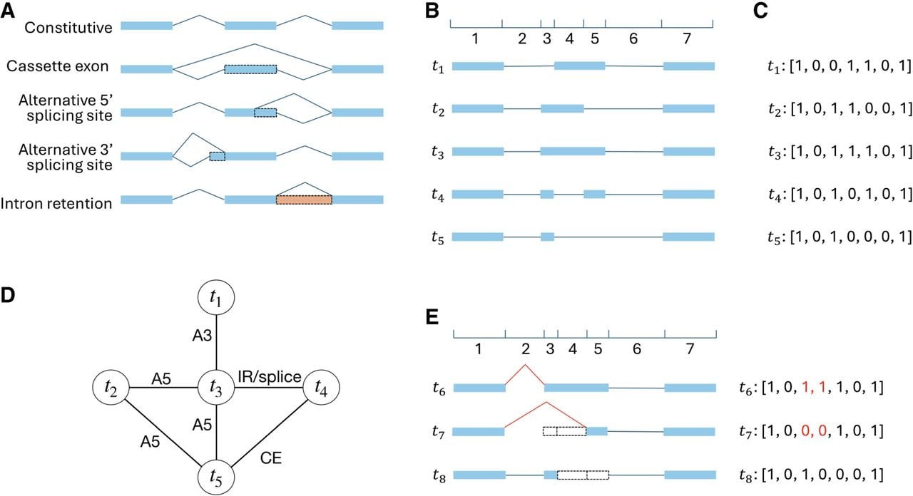
To formalize this model, we represent each transcript as a binary vector encoding the inclusion (1) or exclusion (0) of genomic regions delineated by splice sites (Fig. 1B,C). Two transcripts are connected by an edge if they differ by exactly one AS event. For example, in Figure 1D, transcripts t1 and t3 differ only in the third genomic region and are thus connected. It is easy to identify this event as an A3 event. Importantly, AS events including or excluding multiple consecutive partial exons—such as those arising from alternative 5′ or 3′ splice sites—are treated as single events despite spanning over multiple genomic regions (Fig. 1E). Under this model, all isoforms within a transcript group should form a connected graph, provided none is missing.
When annotated isoforms fail to form a connected graph, it indicates that the annotation may be missing intermediate transcripts. TENNIS identifies such gaps and predicts the minimum number of novel isoforms needed to restore connectivity. We formulate this task as an optimization problem and design an algorithm, TENNIS-SAT, that transforms the subroutine problem into a Boolean satisfiability (SAT) instance: given the binary matrix representation of a transcript group, TENNIS-SAT determines whether adding k novel isoforms suffices to produce a connected graph, and if so, returns their binary representations. For transcript groups with exactly two connected components, an optimal greedy algorithm provides an efficient exact solution. For more complex cases, TENNIS-SAT iteratively tests increasing values of k until a solution is found or computational limits are reached (see Methods for details). We denote the set of single-isoform transcript groups as and the set of multi-isoform transcript groups as . Multi-isoform transcript groups are further classified into (k = 0, 1, …) and groups, meaning they require k additional isoforms or exceed computational resources.
Most transcript groups satisfy the AS evolution model
In a well-annotated transcriptome, we expect most transcript groups to satisfy our evolution-inspired model. To verify, we analyzed 7 transcriptome annotations from 6 model species: human (GRCh38 RefSeq and GENCODE), mouse (GRCm39), Drosophila (dm6), zebrafish (GRCz11), maize (Zm-B73-REFERENCE-NAM-5.0) and Arabidopsis (TAIR10) (Supplemental Table S1). For each transcriptome, we first partition all multi-exon transcripts into transcript groups, as described in Methods. TENNIS is applied to all transcript groups, and according to the outcomes, they are partitioned into 7 categories: .
The statistics are reported in Table 1. We found that 70%–87% of the transcript groups fall into the category, meaning they have just one (multi-exon) transcript. For these groups, transcript isoform diversity arises from distinct TSS and/or TES usage rather than from alternative splicing within a group. This observation aligns well with previous studies that TSS and TES are the major sources of transcriptome diversity (Reyes and Huber 2018), and the selection of TSS and TES is coordinated (Alfonso-Gonzalez et al. 2023; Calvo-Roitberg et al. 2025). Human RefSeq has the lowest single-transcript group rate (70%) whereas human GENCODE has the highest single-transcript group rate (87%). We note that GENCODE has many more transcript groups than RefSeq (145,202 vs. 90,425) but fewer of them are multi-transcript groups (19,425 vs. 26,884). This indicates GENCODE annotated more genes and alternative TSS/TES isoforms but fewer AS isoforms per gene.
Summary statistics of the number of transcript groups in each category
| Species | Annotation | ||||||||
|---|---|---|---|---|---|---|---|---|---|
| Human/GRCh38 | GENCODE | 11,960 (62%) | 4277 (22%) | 1654 (9%) | 676 (3%) | 322 (2%) | 536 (3%) | 19,425 | 125,777 (87%) |
| Human/GRCh38 | RefSeq | 20,852 (78%) | 3951 (15%) | 1169 (4%) | 435 (2%) | 199 (1%) | 278 (1%) | 26,884 | 63,541 (70%) |
| Mouse | GRCm39 | 17,178 (84%) | 2321 (11%) | 599 (3%) | 190 (1%) | 92 (0%) | 102 (0%) | 20,482 | 49,524 (71%) |
| Drosophila | dm6 | 2433 (78%) | 451 (14%) | 116 (4%) | 46 (1%) | 28 (1%) | 42 (1%) | 3116 | 17,938 (85%) |
| Zebrafish | GRCz11 | 7455 (88%) | 673 (8%) | 155 (2%) | 62 (1%) | 21 (0%) | 61 (1%) | 8427 | 41,836 (83%) |
| Maize | NAM-5.0 | 16,799 (88%) | 1612 (8%) | 332 (2%) | 142 (1%) | 53 (0%) | 46 (0%) | 18,984 | 83,398 (81%) |
| Arabidopsis | TAIR10 | 1481 (88%) | 147 (9%) | 33 (2%) | 10 (1%) | 2 (0%) | 2 (0%) | 1675 | 9105 (84%) |
Among the transcript groups with multiple transcripts (i.e., ), the majority (78%–88%, except human/GENCODE) satisfy our model (i.e., are in ), supporting the rationale of this model. Human GENCODE is an outlier, with 62% of transcript groups ending up in . This might be due to a combination of GENCODE over-annotating some transcripts with alternative TSS/TES isoforms and some transcript groups being incomplete. Among transcript groups that do not satisfy our model, the majority are in , that is, for most groups, only one additional isoform is required to make it complete. Lastly, approximately only 1% of transcript groups require more than 4 transcripts to meet our model or time out in 15 minutes for 6 out of the 7 annotations (it is 3% of groups for human GENCODE). Consistent with this observation, for dm6, all transcript groups with an MST-based upper bound of at most 4 were solved within 15 minutes, and the MST-based upper bound is typically equal to or close to the optimal number of novel isoforms across annotations (Supplemental Fig. S1). This suggests that the 15-minute timeout threshold and the default maximum of 4 missing isoforms serve as a sufficient balance between completeness and efficiency for the great majority of transcript groups.
TENNIS-predicted isoforms are validated by long-read RNA-seq data
It is of great interest to test whether TENNIS is able to predict correct novel isoforms. As TENNIS predicts novel/missing isoforms from the reference transcriptome annotations without additional input, if those isoforms can be cross-validated by other data sources such as RNA-seq or external databases, then they are likely to be true positives. In this way, we demonstrate the accuracy and applicability of TENNIS.
We chose the Drosophila transcriptome as an example, which is relatively small and well-studied. We retrieved an assembly of high-depth long-read RNA-seq data from a previously published data set (Alfonso-Gonzalez et al. 2023). We used GffCompare (Pertea and Pertea 2020) to compare the predicted isoforms from TENNIS against this assembly. GffCompare considers two multi-exon isoforms matching if they have the same intron-chain, which is a widely accepted practice. A TENNIS-predicted novel isoform is considered “matched” if it shares the same intron chain as a transcript from a different source. Otherwise, the prediction is considered “unmatched.” In this experiment, we consider “matched” as true-positive and “unmatched” as false-positive. Accordingly, the number of matched predictions is proportional to sensitivity, and the frequency of matched predictions is proportional to precision.
We also set up baseline comparisons through randomized approaches and exon usage-based approaches. Only transcript groups requiring novel isoform prediction, namely those in , were used in these baseline experiments; for dm6 this corresponds to 641 groups, whereas the remaining groups were already complete under our model and therefore did not require prediction. Specifically, within each eligible group, all constitutive exons were always included, and alternative exons were combined to create novel, previously unobserved isoform predictions. We used two random baselines. In the first one, referred to as “Rand1,” one isoform per eligible transcript group is randomly generated; in the second one, termed “RandX,” k novel isoforms per group in were produced, in which the value of k is obtained by TENNIS. To reduce random noise, both “Rand1” and “RandX” experiments were repeated 5 times. Their means and standard deviations were reported. In addition to the random baselines, we designed two more realistic baseline methods that consider exon usage frequencies. We retrieved percent spliced in (PSI) values of alternative exons in Drosophila dm6 annotation from VastDB (Tapial et al. 2017) and computed the average PSI values of each exon across tissues. We designed baseline methods “PSI1” and “PSIX” to construct novel transcripts by selecting exon combinations with the highest product of PSI values. Similar to Rand1 and RandX, PSI1 outputs one transcript per group and PSIX outputs k transcripts per group. These PSI-based methods provide more realistic baselines by considering the likelihood of exon inclusion based on experimental data.
By considering isoforms identified from a real experiment (Alfonso-Gonzalez et al. 2023) as a reference set, we reasoned that the number and rate of isoform predictions matched by those isoforms are good approximations of the relative sensitivities and precisions of methods for isoform prediction. Here, we present a plot of matching rate versus number of matches for TENNIS and the four baseline methods (Fig. 2A).
TENNIS augmentations on the Drosophila transcriptome dm6. (A) The number and percentage of transcript predictions matched by long-read RNA-seq, sorted in descending order of PctIn and then splicing probability score. The color gradient indicates PctIn values, with circles highlighting critical thresholds (PctIn = 0.5, 0.333). Baseline methods include random (Rand1, RandX) and PSI-based (PSI1, PSIX) approaches. Error bars for random baselines represent standard deviation over 5 repetitions. (B) Histogram of PctIn values for predicted transcripts. Three local peaks were observed at 0.333, 0.5, and 1.0 PctIn.
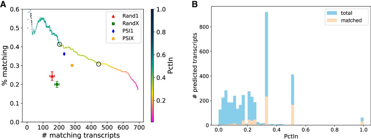
Both randomized baselines have lower matching rates and fewer matched isoforms than TENNIS. The Rand1 baseline outputs 641 multi-exon isoform predictions, in which, averaged over 5 replicates, only 156.6 (24.5%) are matched by long reads. The RandX baseline outputs 933 multi-exon isoform predictions, in which 186.8 (20.0%) isoforms are matched. TENNIS has 640 (resp. 682) matched isoforms at the same matching-rate level as Rand1 (resp. RandX) and matching rates of 46.6% (resp. 45.3%) at the same number of matched isoforms as Rand1 (resp. RandX). The PSI-based baselines substantially outperform the random baselines, in which 232 (36.2%) PSI1 transcripts and 281 (30.1%) PSIX transcripts are matched, demonstrating that exon usage information improves transcript prediction. Nevertheless, TENNIS still outperforms the PSI-based methods. At equivalent numbers of matched isoforms, TENNIS achieves 8.6% higher matching rate than PSI1 and 28.6% higher than PSIX. At equivalent matching-rate levels, TENNIS achieves 36.2% more matching transcripts than PSI1 and 81.5% more than PSIX. Our evolution-inspired model captures additional information beyond exon-usage frequencies. As the PctIn (Percentage In) level of a predicted isoform is defined as the number of SAT solutions containing this isoform divided by the total number of solutions for that transcript group, a higher PctIn level indicates a higher confidence that the predicted isoform indeed is missing from the transcript group. We sorted TENNIS-predicted transcripts in descending order of their PctIn values, and then, if tied, by their splicing probability score.
At the PctIn level of 0.5 and 0.33, TENNIS reported matching rates/numbers of 41.4%/203 and 30.8%/447, respectively (circled points in Fig. 2). Additionally, at the two extremes, TENNIS reported a matching rate of 50% for the intersection of all potential solutions and 693 matched isoforms for the union of all potential solutions. These observations demonstrate that novel transcripts that have a higher chance of being from the evolution trajectory are more likely to be true positives, which supports the evolution-inspired model of TENNIS.
Although the PctIn values indeed range from 0 to 1, their distribution displays significant skewness with discrete peaks occurring at 0.333, 0.50, and a smaller local peak at 1.0 (Fig. 2B). Transcripts with PctIn values of 0.333 (resp. 0.50 or 1.0) may come from a transcript group T in which each has three (resp. two or one) optimal solutions from SAT. Note this concept is different from which describes the number of missing isoforms. In other words, a transcript group T may need only one isoform to form a connected graph (thus, in ), but may have two possible optimal configurations for this isoform by SAT. Correspondingly, transcripts with lower PctIn values are from a transcript group T with more optimal SAT solutions. The latter group is harder to solve, and predicted isoforms from such groups are less favorable. Transcripts with PctIn values of 0.333 (resp. 0.50 or 1.0) have a matching rate of 25% (resp. 40% or 51%), much higher than that of transcripts with lower PctIn values (9.6%). Therefore, we show that PctIn values of 0.5 and 0.333 can generally serve as two good thresholds for filtering TENNIS predictions. We also evaluated TENNIS performance stratified by the number of novel transcripts per group (, , etc.), showing that groups requiring fewer novel isoforms achieve higher matching rates (Supplemental Fig. S2).
TENNIS-predicted novel transcripts have adequate expression levels. We quantified the mean expression levels of matched TENNIS transcripts in several Oxford Nanopore Technologies (ONT) long-read RNA-seq data sets from Alfonso-Gonzalez et al. (2023) (obtained from NCBI Sequence Read Archive [SRA; https://www.ncbi.nlm.nih.gov/sra] accession numbers SRR19355640, SRR19355639, SRR19355636) using Oarfish (Zare Jousheghani et al. 2025). We compared the count per million (CPM) of TENNIS transcripts to CPMs of transcripts from the same transcript group. The mean TENNIS isoforms CPM to group total CPM ratio is 20%. Also, 45% of TENNIS transcripts have higher CPMs than their group average, and 90.4% have at least 10% of their group average CPM (Supplemental Fig. S3).
We also investigated how many of the TENNIS-predicted transcripts preserve open reading frames (ORFs) of their original gene. ORFanage (Varabyou et al. 2023) was employed to compare TENNIS-predicted transcripts with dm6 reference annotation. More than 80% long-read-matched TENNIS transcripts have greater than 90% in-frame length percent identity (ILPI) with their best reference transcript, meaning 90% of the ORFs from the original gene were preserved in-frame, and more than 68% of all TENNIS-predicted transcripts (including those unmatched by long reads) preserve 90% of the original ORFs (Supplemental Fig. S4). These results imply that TENNIS transcripts may constitute a substantial proportion of the transcriptome in real samples.
Notably, not all genes or transcripts are expressed, and not all expressed transcripts are captured by sequencing. Hence, using assemblies and quantification from real RNA-seq as a ground truth tends to underestimate the total number of true-positive genes and/or transcripts. In other words, transcript predictions unmatched by an assembly may be false-positive predictions or may be unexpressed or unsequenced in the experiments. To estimate the coverage of genes in our “ground-truth” (namely, the assembly from Alfonso-Gonzalez et al. 2023), we compared it with dm6 annotations, in addition to TENNIS outputs. GffCompare (Pertea and Pertea 2020) reported this long-read assembly overlaps with only 54.0% loci (based on exon overlapping) in dm6 annotation and 63.0% loci in TENNIS. Hence, the number of true positives is most likely underestimated for TENNIS to a noticeable level.
TENNIS accurately retrieves isoforms in a removal simulation
To further validate TENNIS’s ability to detect missing transcripts, we conducted a simulation using a removal and retrieval approach. From genes containing three or more annotated isoforms, we randomly removed one isoform. The removed isoform could not be the shortest isoform, and its removal could not reduce the total number of exons (i.e., the exon spliced out in all other isoforms) in the group, so that retrieval of this isoform is not impossible. This experimental design aimed to assess both the matching rate and the number of matched transcripts of TENNIS in identifying missing transcripts. GffCompare was used for evaluation and the removed transcripts are regarded as ground truth.
A total of 796 multi-isoform groups were used for this removal simulation. TENNIS classified the 796 groups to 262(33%) , 342(43%) , 102(13%) , 30(4%) , 23(3%) , and 37(5%) groups. The percentages of all classes increased, compared to Table 1. This is expected as we removed one isoform from each group. The presence of groups indicates that some groups have a more “connected” graph and that not all non-terminal vertices are cut vertices. Besides, those 796 groups do not necessarily satisfy the evolution model prior to the removal. Therefore, the missing isoform identification problem is further complicated.
TENNIS achieved high matching rates and numbers of matched transcripts, which are considerably better than those of baseline approaches, in this simulated removal-and-retrieval experiment (Fig. 3A). At PctIn values of 0.5 or 0.333, TENNIS has a matching rate of 40.6% or 27.9% and 202 or 329 matched transcripts. The matching rates and numbers of matched transcripts for Rand1 are 21.8% and 108.2, whereas those for RandX are 16.6% and 120.6, averaged over 5 replicates. The matching rates and numbers of matched transcripts for PSI1 are 27.2% and 135, whereas those for PSIX are 20.6% and 150. At an equivalent matching-rate level or number of matched transcripts, TENNIS substantially outperforms all four baseline methods, as demonstrated by its curve lying above the baseline data points in Figure 3A.
TENNIS outperforms baseline methods in transcript-retrieval simulations. (A) The number and percentage of transcript predictions validated against exactly removed isoforms. The color gradient indicates PctIn values, with circles highlighting critical thresholds (PctIn = 0.5, 0.333). Baseline methods include random (Rand1, RandX) and PSI-based (PSI1, PSIX) approaches. Error bars represent standard deviation over 5 repetitions. (B) Histogram of PctIn values for predicted transcripts validated against exactly removed isoforms. (C) The number and percentage of transcript predictions validated against combined ground truth (exactly removed isoforms + long-read RNA-seq assembly), using the same color scheme as panel A. (D) Histogram of PctIn values for predicted transcripts validated against the combined ground truth.
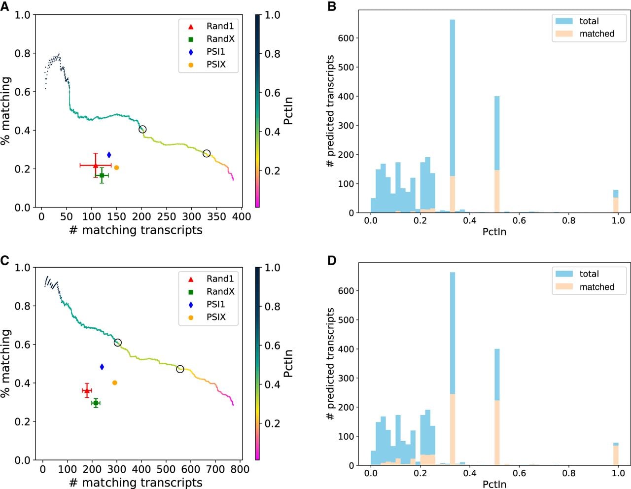
Considering the presence of multiple solutions and the potential incompleteness of annotations, we also evaluated the predictions using the combined ground truth, that is, union of removed transcripts and the long-read RNA-seq assembly (Fig. 3C). Hence, previously predicted transcripts that are not matched by the exactly removed transcripts could potentially be validated by real sequencing data. At a PctIn level of 0.5 (resp. 0.333), TENNIS successfully predicts 304 (resp. 556) matched isoforms with a matching rate of 61.0% (resp. 47.1%). The baseline approaches Rand1 and RandX respectively identified only 179.4 and 215.2 matched isoforms with matching rates of 36.1% and 29.6%, averaged across 5 replicates. PSI1 had 240 (48.3%) transcripts matched and PSIX had 292 (40.1%) transcripts matched. At an equivalent matching-rate level or number of matched transcripts, the performance of TENNIS is again higher than that of those four baselines.
The distribution of PctIn values mirrors the pattern observed in real data, exhibiting local peaks at 0.33, 0.5, and 1.0 (Figs. 3B,D). The matching rates of isoforms with those PctIn values are 19%, 37%, 67% if validated by exact removed isoforms, and 37%, 56%, 87% if validated by combined ground truth.
We also evaluated TENNIS performance stratified by the number of novel transcripts per group (, , etc.). Similar to the case with real data, when a group requires fewer novel isoforms, the matching rates are higher (Supplemental Figs. S5 and S6). Additionally, more complex simulation experiments were performed by extending the simulation to remove 2 or 3 transcripts per group, and TENNIS consistently outperformed all baseline methods in these more challenging scenarios (Supplemental Fig. S7).
Cross-validation on human annotations
We investigated whether TENNIS predictions on one annotation can be validated using another annotation of the same species. We conducted this experiment using human GENCODE and RefSeq annotations. As GffCompare considers multi-exon transcripts with identical intron-chains as “matching,” we removed transcript groups that do not share identical “first-exon donor and last-exon acceptor” combinations between RefSeq and GENCODE, because TENNIS-predicted isoforms from those groups will never match with the other annotation.
We compared TENNIS-predicted transcripts from GENCODE (referred to as TENNIS_Gencode) with human RefSeq annotation. At the level of PctIn = 0.5, TENNIS_Gencode has 672 transcripts matched/26.78% matching rate with RefSeq annotation. An additional 528 TENNIS_Gencode transcripts (21%) matched with TENNIS_RefSeq (TENNIS-predicted transcripts from RefSeq), meaning those 528 transcripts are potentially missing from both annotations and can be recovered by our method. Those results indicate that a substantial number of TENNIS-predicted transcripts can be validated using a different annotation data set. Serving as a comparison baseline, 15.3% of multi-exon transcripts in GENCODE annotation and 42.5% in RefSeq annotation match each other.
Discussion
A comprehensive transcriptome annotation is essential for many bioinformatics and biomedical studies. Although significant resources have been invested in improving these annotations through the invention of new methods, pipelines, and manual curations, the great majority of these annotations, if not all, are data-driven (Aken et al. 2016; Pertea et al. 2018; Li et al. 2021; Morales et al. 2022). Little attention has been paid to modeling the annotated isoforms particularly from an evolutionary perspective. We fill this critical gap with TENNIS, an evolution-inspired model for characterizing annotated transcripts, together with an algorithm that infers missing isoforms in an annotation. The model of TENNIS is simple: isoforms in a transcript group are connected in a single component using the four basic AS events, provided no isoform is missing. When this condition is not satisfied, TENNIS seeks the minimum number of isoforms to make them connected, using a novel SAT formulation that guarantees to find all optimal solutions.
We analyzed seven transcriptome annotations of model organisms using TENNIS. We showed that the majority of transcript groups are single-isoform, accounting for about 80% of all multi-exon groups. The evolution-inspired model is satisfied by 62%–88% of transcript groups in various species’ annotations, supporting the propositions of our model. We also evaluated the validity of TENNIS isoform predictions by comparing them with a long-read RNA-seq assembly and through a simulation experiment of removal and retrieval. In both settings, TENNIS outperformed the randomized and PSI-based baseline methods. After controlling the same number of matched transcripts or matching rate, TENNIS showed approximately a 70%–200% increase in matching rate and 250%–330% increase in the number of matched transcripts over the baselines in the experiments. Furthermore, the analysis revealed that if an isoform appears in multiple optimal solutions with a higher percentage (PctIn), then it is more likely to represent a true isoform. The PctIn metric can thus serve as an effective criterion for filtering predicted isoforms.
The missing isoforms identified by TENNIS should be interpreted as transcripts that are plausibly annotatable under our model. Their identification does not imply that these isoforms are actively expressed in extant species. Rather, it is entirely possible that some of these transcripts were expressed historically but have since been lost, silenced, or otherwise suppressed during evolution in specific lineages or clades. Empirical validation of these predicted isoforms should rely on experimental evidence, such as assembling and quantifying RNA-seq data.
Although TENNIS is inspired by evolutionary principles, we note that it does not directly compare transcriptomes across species. Cross-species validation of predicted isoforms remains challenging because homologous genes may have divergent transcript structures and sequences. Genes that are highly conserved tend to have conserved transcripts across species, whereas less conserved genes may have different structures that are difficult to align. Nevertheless, TENNIS provides meaningful insights when comparing different annotations of the same species, as demonstrated by our cross-annotation validation between GENCODE and RefSeq. A direct cross-species isoform evolution analysis would be an interesting direction for future work.
TENNIS is best applied when a gene has multiple isoforms with the same transcription start site (TSS) and transcription end site (TES). This condition ensures that the transcripts originate from the same pre-mRNA and their diversity results purely from alternative splicing. For under-annotated genomes, in which many genes have only one annotated transcript and are hence categorized as , users may benefit from performing RNA-seq assembly prior to applying TENNIS, thereby leveraging sequencing data to first identify multiple isoforms per gene.
The assumption made by TENNIS is minimal, yet demonstrates strong prediction capability in identifying missing isoforms. It therefore holds great potential to model complex evolutionary trajectories. A promising future enhancement for TENNIS is the integration of additional prior knowledge and features related to (AS) events, such as the lengths and sequences of introns/exons, their splicing patterns, and conservation of ORFs of original genes. Previous studies have established that constitutive exons typically exhibit greater lengths and are flanked by shorter introns, whereas alternatively spliced exons are more likely to be shorter and accompanied by longer introns (Ast 2004; Kim et al. 2007b; Lev-Maor et al. 2007). Also, Lev-Maor et al. (2007) revealed a positive correlation between expression level and evolutionarily conserved transcripts, which are often ancestral. As a mathematical model to characterize observed isoforms, TENNIS fills the research gap of AS evolution and provides valuable insights for various research areas including alternative splicing mechanisms, comparative transcriptomics, and phylo-transcriptomics studies.
Methods
An evolution-inspired model
TENNIS models the evolution of alternative splicing (AS) within a transcript group (defined below) based on two premises: (1) AS isoforms evolve sequentially, with each isoform being derived from a predecessor; and (2) each isoform must originate from its parent through a single AS event (CE, A3, A5, or IR) per evolutionary step. The rationale behind the second premise is that AS events arise independently through mutations in splicing sites or regulatory elements and it is less likely to have two mutations occur simultaneously (Ast 2004; Zhang et al. 2017). Consequently, all isoforms of a transcript group should be connected via single AS events. If not, then it indicates that isoform(s) are missing from the annotation or have lost function and therefore are not present in the current annotation.
The framework of TENNIS is as follows. It takes a transcriptome or an assembly, that is, a set of annotated or assembled transcripts in GTF format, as input. It first partitions all transcripts into transcript groups (defined below). Within each group, it constructs the evolutionary relationship using a graph, determines evidence of missing isoforms, and if evidence is present, identifies the missing isoforms.
We focused on analyzing AS isoforms originating from the same pre-mRNA. That is, TENNIS groups transcripts that share the same alternative transcription start site (TSS) and alternative transcription end site (TES) together, referred to as a “transcript group.” We denote by the set of transcript groups with just a single transcript, and by the set of transcript groups with two or more transcripts. Figure 1B shows an example of a transcript group with 5 transcripts. Although TSS and TES are two events that also produce diverse transcripts, the pre-mRNAs are already different for transcripts with such events (Marasco and Kornblihtt 2023). Hence, the AS processes are more different between transcripts with alternative TSS or TES (Reyes and Huber 2018; Alfonso-Gonzalez et al. 2023).
Next, TENNIS builds a graph for each transcript group. In the graph, the collection of nodes represents all isoforms and the collection of edges represents whether two isoforms are convertible via a single AS event. For example, Figure 1D illustrates the graph for transcripts in Figure 1B. Details of the construction of graphs are described in the next subsection. We say that a transcript group does not present evidence of missing isoform(s) if the graph is connected (i.e., the group consists of a single connected component). Otherwise, TENNIS recruits a minimal number of additional nodes to make all components connected. These reconstructed nodes/transcripts are regarded as missing isoforms. This step is modeled as an optimization problem and solved by transforming it into a satisfiability (SAT) formulation, detailed in the TENNIS-SAT section below.
Constructing evolution trajectory and identifying missing isoforms
Let T be a transcript group. TENNIS encodes each isoform in T as a binary vector, depicting exonic or intronic regions. First, genomic coordinates of all splicing sites of all isoforms in T are collected and then the genome is split into smaller regions according to those coordinates (Fig. 1B). Let n be the number of resulting genomic regions. Clearly, each exon or intron spans either one region or several consecutive regions. Hence, every isoform in T can be described using indices of spliced-in regions (i.e. exonic regions) and indices of spliced-out regions (i.e., intronic regions). Therefore, by encoding the exonic region as 1 and intronic regions as 0, an isoform is encoded as a length-n binary vector. For example, a 1 at position i of the binary vector means the ith genomic region is covered by an exon in this isoform and vice versa (see Fig. 1C). Assume T contains m isoforms. Then T can be represented as an m × n binary matrix, denoted as M.
The benefits of binary encoding of isoforms are that, besides clarity and conciseness, all simple AS events can be represented as the flip of a bit or several consecutive bits. While an exon is split into multiple smaller regions (in this case, called partial-exons) due to A3/A5 events in another isoform, this exon is accordingly coded as multiple 1s. Partial-introns are defined likewise. Hence, the A3/A5 event can be represented as a flip of the bits of those corresponding partial-exons to partial-introns. CE and IR are also represented as 1-to-0 or 0-to-1 flips. Equivalently, all simple AS events can be considered as the inclusion or exclusion of one or multiple consecutive regions.
Given an m × n binary matrix M representing a transcript group, a graph will be constructed. Each annotated isoform is denoted as a vertex. An edge may be added between two vertices if their isoforms can convert to each other by one AS event, that is, a flip of consecutive 0s to 1s or consecutive 1s to 0s. Edges are undirected, because 0-to-1 and 1-to-0 flips are symmetric. This also reflects the invertible property of the basic events.
Provided no transcript is missing, all vertices should be in one connected component. In this case, we say that transcript group T satisfies our evolution-inspired model, and call T a transcript group in . Otherwise, one or more isoforms are said to be missing from T. It is important to note that, due to the minimality of our model, neither direction of the reasoning is decisive; that is, it is possible that T misses some isoforms but the resulting graph remains connected, and it is also possible that the graph is not connected but T does not miss any unannotated isoform.
In the case that the graph contains more than one connected component, TENNIS will reconstruct missing isoforms. We formulate this task as an optimization problem, that is, to find a minimum number of isoforms such that adding them to T results in a graph with just one connected component. This is a parsimonious assumption—that a minimal number of isoforms are missing from the annotations. We design an algorithm, termed TENNIS-SAT (M, k), described in detail in the next section. TENNIS-SAT takes matrix M and an integer k ≥ 1 as input, and answers if adding k isoforms suffices to make the resulting graph connected, and if yes, also returns the binary representation of the k additional isoforms. Using TENNIS-SAT as a subroutine, starting with k = 1, TENNIS employs an iterative approach that calls TENNIS-SAT(M, k) in each iteration and increases k, until either the subroutine returns yes (and the k isoforms) or a maximum iteration number is reached. As a compromise of computational time and accuracy, the default maximum iterations, which is also the maximum number of missing isoforms that TENNIS attempts to reconstruct, is 4. According to our experiments, with this threshold, the model can explain more than 97% of the investigated transcript groups (Table 1). Transcript group T will be assigned to a category , if TENNIS determines that a minimum of k transcripts are missing from T, k = 1, 2, 3, 4. T will be assigned to category if the maximum iteration is reached, which means T misses more than 4 transcripts, or TENNIS fails to finish in 15 minutes. Optionally, users can replace this fixed default with an MST-based per-group upper bound, as described later. Additional computational considerations on why conserved positions cannot simply be collapsed are discussed in Supplemental Note S4.
It is common that multiple optimal solutions exist. This means, for a transcript group T in , different sets of k isoforms may make the resulting graph connected. TENNIS is able to return all optimal solutions. This offers an additional critical signal to decide if a constructed missing isoform is correct or not. The intuition is that if there are multiple optimal solutions, and an isoform appears in all of them, then it is more likely to be truly missed than isoforms that appear in only one solution. Therefore, for each reconstructed isoform in the union of all optimal solutions, we introduce a measure “Percentage In (PctIn),” defined as the number of solutions containing this isoform divided by the total number of solutions.
TENNIS-SAT
Given an m × n binary matrix M representing all isoforms in a transcript group T, and an integer k representing the maximum number of missing isoforms allowed to be added, we use a SAT formulation to decide if adding k isoforms is sufficient to connect the graph. Similar to existing isoforms, the unknown novel isoforms are represented as a vector of binary variables. For simplicity, they are appended to M, and all isoforms are represented by rows in M. This means that Mi is a length-n vector of known binary values for i = 1, …, m, whereas Mi is a length-n vector of unknown binary variables for i = m + 1, …, m + k.
As the aim is to construct a connected graph, the presence of a spanning tree in the graph is necessary and sufficient. The spanning tree can be more efficiently represented in SAT by treating it as a rooted tree. In the constructed tree, each vertex denotes a row of M (i.e., one isoform) and this tree should have m + k vertices and at most m + k levels. Otherwise, the problem is infeasible. The high-level idea of the SAT formulation is trying to put each vertex, including both given and missing ones, to a certain level of the tree and construct their parent–child relationship. It is worth noting that such a parent–child relationship is solely for the convenience of construction, it does not indicate the direction of evolution — recall that our model is an undirected graph that primarily concerns about the presence/absence of isoforms, no effort has been made to infer the actual evolutionary trajectory.
We now provide the implementation details for the above idea. Recall that an SAT formulation consists of a set of boolean/binary variables and a conjunction of clauses where each clause is a disjunction of literals (boolean variables or their negations). We first introduce boolean variable Di,j to denote whether an edge exists between vertex i and vertex j, i ≠ j. So Di,j is True if and only if the ith isoform is derivable from the jth isoform via exactly one simple AS event. Let a helper binary variable di,j,k denote the number of (extra) events needed to convert Mi,k from Mj,k (i ≠ j), that is, flipping the bit of the kth region. As we only permit one AS event between direct parent–child isoforms, Di,j is set to True if and only if exactly one variable in {di,j,k| 1 ≤ k ≤ n} is True. Enforcing the condition “exactly one variable in a set must be True” can be implemented as SAT clauses detailed in Supplemental Note S1.
Consider a simplified case when all exons are represented by exactly one region, that is, no partial-exons. Then di,j,k is set to True if and only if Mi,k ≠ Mj,k (Supplemental Note S2). However, when partial-exons exist, skipping multiple consecutive partial-exons is also regarded as one event because it takes the same number of splicing to skip one exon or multiple consecutive partial-exons (Fig. 1E). Thus, we set di,j,k to True, if and only if both conditions are true: (1) Mi,k ≠ Mj,k; and (2) Mi,k ≠ Mi,k−1 or Mj,k ≠ Mj,k−1, 2 ≤ k ≤ n; (second condition not required when k = 1). Otherwise the difference between Mi,k and Mj,k has been compensated at or before position k − 1, so the penalty should not be double-counted. Those two conditions can be modeled by clauses in Supplemental Note S3.
After properly representing edges with Di,j, we can fit vertices into a tree. Let boolean variable Li,j denote whether vertex i is on level j of this tree. Li,j should satisfy the following constraints: First, a vertex appears exactly once in the tree, which means for the ith isoform, exactly one of the variables in is set to True. Second, exactly one vertex, that is, the root, is on level 1, namely, exactly one variable in is True. Both require the constraint “exactly one variable in a set is True,” which again can be modeled with the approach in Supplemental Note S1.
Next, we add constraints governing the spanning tree edges. The idea is that if a vertex i is present at level g (g ≥ 2), then there must exist a node j on level g − 1 that has an edge connecting to vertex i, namely, Di,j is True. Let binary variable Ci,j,g denote if vertex i is on level g of the tree and is preceded by vertex j on level g − 1 through one simple AS event of edge Di,j. Therefore, Ci,j,g can only be set to True if all three variables Di,j, Li,g, and Lj,g−1 are True. However, the reverse direction does not always hold because Di,j may be true for different pairs of vertices i and j. Intuitively, a vertex i can have multiple potential parents in the graph, but we only choose one in the constructed spanning tree. These constraints can be modeled by 3 SAT clauses:
TENNIS implements the SAT formulation via the pySAT interface (Ignatiev et al. 2018) and solves the problems using the Glucose SAT solver (Audemard and Simon 2018). We configure it to time out after 15 minutes to balance computational efficiency and accuracy.
Optimal greedy algorithm for two connected components
When a transcript group has exactly two connected components, an optimal solution can be computed using a simple greedy algorithm without resorting to the SAT formulation. This algorithm is both faster and guaranteed to find the minimum number of missing isoforms needed to connect the two components.
Let C1 and C2 be the two connected components in the graph constructed from matrix M. The optimal greedy algorithm proceeds by first computing the pairwise distance d(i, j) for all pairs, in which i ∈ C1 and j ∈ C2. Here, counts the number of AS events separating isoforms i and j, as defined in the TENNIS-SAT formulation above. Next, the algorithm identifies the minimum distance d(i, j) across all such pairs (d* ≥ 2, otherwise C1 and C2 would be connected). The minimum number of missing isoforms needed to connect the two components is then d* − 1. Finally, for each pair (i′, j′) achieving the minimum distance d*, the algorithm enumerates all possible paths of intermediate isoforms connecting i′ to j′, in which each path (excluding node i′ and j′) represents a distinct optimal solution. The minimal number of novel transcripts needed to connect the two components is the same as that needed to connect transcripts i′ and j′. When partial-exons do not exist, we can connect i′ and j′ through a path of a series of single-event edges by sequentially flipping the d* differing bits one at a time. This creates d* − 1 intermediate isoforms, each differing from its neighbors by exactly one bit flip (representing one simple AS event), thereby yielding one optimal solution. If partial-exons exist (defined in the above formulation of TENNIS-SAT as consecutive bits), we flip differing consecutive bits instead of one bit each time. Hence, the above d* − 1 intermediate-isoform solution still holds.
Upper bound computation for novel transcripts
To balance computational efficiency and performance, TENNIS uses a fixed upper bound of 4 novel isoforms by default. Optionally, the upper bound of the number of novel transcripts in a group can be computed by an algorithm based on the minimal spanning tree (MST).
We construct a weighted hypergraph H, in which each node represents a connected component, and edges between nodes are weighted by the minimum distance between any two isoforms from the respective components. A minimum spanning tree (MST) of H guarantees an efficient way to connect all components using an upper bound on the number of novel isoforms. If the MST has edges with weights w1, w2, …, wc−1 (where c is the number of connected components and wi is at least 2), then the upper bound is . This bound is guaranteed to be achievable because we can independently apply the two-component greedy algorithm to connect components according to the MST structure.
Computing the MST-based upper bounds has a few benefits. First, it enables per-group flexibility: rather than applying a single fixed global cutoff (e.g., k ≤ 4), users can set tighter or looser iteration limits based on group-level complexity such as the number of annotated isoforms or exons. Second, when the bound is 1, the greedy algorithm is guaranteed to find the optimum and the SAT solver is bypassed entirely, saving computation. Third, when the SAT solver times out before converging, the precomputed bound characterizes the remaining search space: without it, a timeout leaves open whether the current k is simply infeasible or whether more time would suffice; with it, users can make an informed decision to relax the time limit or switch to the greedy solver. The greedy solver is attempted first for all cases; if it succeeds, the result is returned immediately. Otherwise, the computed upper bound guides the iterative SAT solver to focus on the feasible solution space.
Splicing probability scoring for predicted transcripts
To further refine the ranking of TENNIS-predicted isoforms, we computed a splicing probability score for each predicted transcript based on exon inclusion rates. This score quantifies the likelihood of an isoform given the included exons. The scoring scheme takes the predicted transcripts and the collected experimentally measured PSI (percent spliced-in) values of exons as inputs.
Given an m × n binary matrix M representing all isoforms in a transcript group T, let Mi represent the i-th isoform as a binary vector of length n, and let j index the exons such that Mi,j ∈ {0, 1} indicates the inclusion of exon j. Let pj denote the inclusion probability (PSI) of the jth exon. The splicing probability sp(Mi) is computed as:
Code availability
TENNIS is implemented in Python and is freely available as open-source software under the BSD-3-Clause license at GitHub (https://github.com/Shao-Group/tennis). Scripts, documentation, and data descriptions for reproducing the experiments in this manuscript are available at GitHub (https://github.com/Shao-Group/tennis-test) and as Supplemental Code.
Competing interest statement
The authors declare no competing interests.
Acknowledgments
The authors thank Tasfia Zahin for help in data collection and processing. This work is supported by the U.S. National Science Foundation (2145171 to M.S.) and by the U.S. National Institutes of Health (R01HG011065 to M.S.).
Author contributions: X.C.Z. and M.S. conceived of the project. X.C.Z., K.C., and M.S. designed the algorithm. X.C.Z. and K.C. implemented the software. X.C.Z. and I.M.K. performed the experiments. All authors analyzed the results. All authors wrote, reviewed, and approved the manuscript. M.S. supervised the project.
Footnotes
[1] Supplementary material [Supplemental material is available for this article.]
[2] Article published online before print. Article, supplemental material, and publication date are at https://www.genome.org/cgi/doi/10.1101/gr.280661.125.
[3] Freely available online through the Genome Research Open Access option.
References
- ↵Aken BL, Ayling S, Barrell D, Clarke L, Curwen V, Fairley S, Banet JF, Billis K, Girón CG, Hourlier T, 2016. The Ensembl gene annotation system. Database 2016: baw093. 10.1093/database/baw093
- ↵Alfonso-Gonzalez C, Legnini I, Holec S, Arrigoni L, Ozbulut HC, Mateos F, Koppstein D, Rybak-Wolf A, Bönisch U, Rajewsky N, 2023. Sites of transcription initiation drive mRNA isoform selection. Cell 186: 2438–2455.e22. 10.1016/j.cell.2023.04.012
- ↵Ast G. 2004. How did alternative splicing evolve? Nat Rev Genet 5: 773–782. 10.1038/nrg1451
- ↵Audemard G, Simon L. 2018. On the Glucose SAT solver. Int J Artif Intell Tools 27: 1840001. 10.1142/S0218213018400018
- ↵Birzele F, Csaba G, Zimmer R. 2008. Alternative splicing and protein structure evolution. Nucleic Acids Res 36: 550–558. 10.1093/nar/gkm1054
- ↵Calvo-Roitberg E, Carroll CL, Kim G, Sanabria V, Venev SV, Mick ST, Paquette JD, Uriostegui-Arcos M, Dekker J, Fiszbein A, 2025. mRNA initiation and termination are spatially coordinated. Science 390: eado8279. 10.1126/science.ado8279
- ↵Chen M, Manley JL. 2009. Mechanisms of alternative splicing regulation: insights from molecular and genomics approaches. Nat Rev Mol Cell Biol 10: 741–754. 10.1038/nrm2777
- ↵Hoyos LE, Abdel-Wahab O. 2018. Cancer-specific splicing changes and the potential for splicing-derived neoantigens. Cancer Cell 34: 181–183. 10.1016/j.ccell.2018.07.008
- ↵Ignatiev A, Morgado A, Marques-Silva J. 2018. PySAT: A Python toolkit for prototyping with SAT oracles. In Theory and Applications of Satisfiability Testing - SAT 2018 (ed. Beyersdorff O, Wintersteiger C), Lecture Notes in Computer Science, Vol. 10929, pp. 428–437. Springer, Cham, Switzerland. 10.1007/978-3-319-94144-8_26
- ↵Keren H, Lev-Maor G, Ast G. 2010. Alternative splicing and evolution: diversification, exon definition and function. Nat Rev Genet 11: 345–355. 10.1038/nrg2776
- ↵Kim E, Goren A, Ast G. 2007a. Alternative splicing: current perspectives. BioEssays 30: 38–47. 10.1002/bies.20692
- ↵Kim E, Magen A, Ast G. 2007b. Different levels of alternative splicing among eukaryotes. Nucleic Acids Res 35: 125–131. 10.1093/nar/gkl924
- ↵Leung SK, Jeffries AR, Castanho I, Jordan BT, Moore K, Davies JP, Dempster EL, Bray NJ, O’Neill P, Tseng E, 2021. Full-length transcript sequencing of human and mouse cerebral cortex identifies widespread isoform diversity and alternative splicing. Cell Rep 37: 110022. 10.1016/j.celrep.2021.110022
- ↵Lev-Maor G, Goren A, Sela N, Kim E, Keren H, Doron-Faigenboim A, Leibman-Barak S, Pupko T, Ast G. 2007. The “alternative” choice of constitutive exons throughout evolution. PLoS Genet 3: e203. 10.1371/journal.pgen.0030203
- ↵Li W, O’Neill KR, Haft DH, DiCuccio M, Chetvernin V, Badretdin A, Coulouris G, Chitsaz F, Derbyshire MK, Durkin AS, 2021. RefSeq: expanding the prokaryotic genome annotation pipeline reach with protein family model curation. Nucleic Acids Res 49: D1020–D1028. 10.1093/nar/gkaa1105
- ↵Marasco LE, Kornblihtt AR. 2023. The physiology of alternative splicing. Nat Rev Mol Cell Biol 24: 242–254. 10.1038/s41580-022-00545-z
- ↵Mattick JS, Amaral PP, Carninci P, Carpenter S, Chang HY, Chen LL, Chen R, Dean C, Dinger ME, Fitzgerald KA, 2023. Long non-coding RNAs: definitions, functions, challenges and recommendations. Nat Rev Mol Cell Biol 24: 430–447. 10.1038/s41580-022-00566-8
- ↵Morales J, Pujar S, Loveland JE, Astashyn A, Bennett R, Berry A, Cox E, Davidson C, Ermolaeva O, Farrell CM, 2022. A joint NCBI and EMBL-EBI transcript set for clinical genomics and research. Nature 604: 310–315. 10.1038/s41586-022-04558-8
- ↵Nurk S, Koren S, Rhie A, Rautiainen M, Bzikadze AV, Mikheenko A, Vollger MR, Altemose N, Uralsky L, Gershman A, 2022. The complete sequence of a human genome. Science 376: 44–53. 10.1126/science.abj6987
- ↵Pan Q, Shai O, Lee LJ, Frey BJ, Blencowe BJ. 2008. Deep surveying of alternative splicing complexity in the human transcriptome by high-throughput sequencing. Nat Genet 40: 1413–1415. 10.1038/ng.259
- ↵Pertea G, Pertea M. 2020. GFF utilities: GffRead and GffCompare. F1000 Res 9: 304. 10.12688/f1000research.23297.1
- ↵Pertea M, Shumate A, Pertea G, Varabyou A, Breitwieser FP, Chang YC, Madugundu AK, Pandey A, Salzberg SL. 2018. CHESS: a new human gene catalog curated from thousands of large-scale RNA sequencing experiments reveals extensive transcriptional noise. Genome Biol 19: 208. 10.1186/s13059-018-1590-2
- ↵Raghavan V, Kraft L, Mesny F, Rigerte L. 2022. A simple guide to de novo transcriptome assembly and annotation. Brief Bioinform 23: bbab563. 10.1093/bib/bbab563
- ↵Reyes A, Huber W. 2018. Alternative start and termination sites of transcription drive most transcript isoform differences across human tissues. Nucleic Acids Res 46: 582–592. 10.1093/nar/gkx1165
- ↵Salzberg SL. 2019. Next-generation genome annotation: we still struggle to get it right. Genome Biol 20: 92. 10.1186/s13059-019-1715-2
- ↵Schneider VA, Graves-Lindsay T, Howe K, Bouk N, Chen HC, Kitts PA, Murphy TD, Pruitt KD, Thibaud-Nissen F, Albracht D, 2017. Evaluation of GRCh38 and de novo haploid genome assemblies demonstrates the enduring quality of the reference assembly. Genome Res 27: 849–864. 10.1101/gr.213611.116
- ↵Scotti MM, Swanson MS. 2016. RNA mis-splicing in disease. Nat Rev Genet 17: 19–32. 10.1038/nrg.2015.3
- ↵Singh P, Ahi EP. 2022. The importance of alternative splicing in adaptive evolution. Mol Ecol 31: 1928–1938. 10.1111/mec.16377
- ↵Statello L, Guo CJ, Chen LL, Huarte M. 2021. Gene regulation by long non-coding RNAs and its biological functions. Nat Rev Mol Cell Biol 22: 96–118. 10.1038/s41580-020-00315-9
- ↵Steward RA, de Jong MA, Oostra V, Wheat CW. 2022. Alternative splicing in seasonal plasticity and the potential for adaptation to environmental change. Nat Commun 13: 755. 10.1038/s41467-022-28306-8
- ↵Sugnet CW, Kent WJ, Ares M, Haussler D. 2004. Transcriptome and genome conservation of alternative splicing events in humans and mice. In Pac Symp Biocomput 2004: pp. 66–77. 10.1142/9789812704856_0007
- ↵Tao Y, Zhang Q, Wang H, Yang X, Mu H. 2024. Alternative splicing and related RNA binding proteins in human health and disease. Signal Transduct Target Ther 9: 26. 10.1038/s41392-024-01734-2
- ↵Tapial J, Ha KC, Sterne-Weiler T, Gohr A, Braunschweig U, Hermoso-Pulido A, Quesnel-Vallières M, Permanyer J, Sodaei R, Marquez Y, 2017. An atlas of alternative splicing profiles and functional associations reveals new regulatory programs and genes that simultaneously express multiple major isoforms. Genome Res 27: 1759–1768. 10.1101/gr.220962.117
- ↵Tian L, Jabbari JS, Thijssen R, Gouil Q, Amarasinghe SL, Voogd O, Kariyawasam H, Du MRM, Schuster J, Wang C, 2021. Comprehensive characterization of single-cell full-length isoforms in human and mouse with long-read sequencing. Genome Biol 22: 310. 10.1186/s13059-021-02525-6
- ↵Varabyou A, Erdogdu B, Salzberg SL, Pertea M. 2023. Investigating open reading frames in known and novel transcripts using ORFanage. Nat Comput Sci 3: 700–708. 10.1038/s43588-023-00496-1
- ↵Wang ET, Sandberg R, Luo S, Khrebtukova I, Zhang L, Mayr C, Kingsmore SF, Schroth GP, Burge CB. 2008. Alternative isoform regulation in human tissue transcriptomes. Nature 456: 470–476. 10.1038/nature07509
- ↵Wang Y, Liu J, Huang B, Xu YM, Li J, Huang LF, Lin J, Zhang J, Min QH, Yang WM, 2014. Mechanism of alternative splicing and its regulation. Biomed Rep 3: 152–158. 10.3892/br.2014.407
- ↵Wright CJ, Smith CWJ, Jiggins CD. 2022. Alternative splicing as a source of phenotypic diversity. Nat Rev Genet 23: 697–710. 10.1038/s41576-022-00514-4
- ↵Zare Jousheghani Z, Singh NP, Patro R. 2025. Oarfish: enhanced probabilistic modeling leads to improved accuracy in long read transcriptome quantification. Bioinformatics 41: i304–i313. 10.1093/bioinformatics/btaf240
- ↵Zerbino DR, Frankish A, Flicek P. 2020. Progress, challenges, and surprises in annotating the human genome. Annu Rev Genomics Hum Genet 21: 55–79. 10.1146/annurev-genom-121119-083418
- ↵Zhang SJ, Wang C, Yan S, Fu A, Luan X, Li Y, Sunny Shen Q, Zhong X, Chen JY, Wang X, 2017. Isoform evolution in primates through independent combination of alternative RNA processing events. Mol Biol Evol 34: 2453–2468. 10.1093/molbev/msx212
- ↵Zhang D, Guelfi S, Garcia-Ruiz S, Costa B, Reynolds RH, D’Sa K, Liu W, Courtin T, Peterson A, Jaffe AE, 2020. Incomplete annotation has a disproportionate impact on our understanding of Mendelian and complex neurogenetic disorders. Sci Adv 6: eaay8299. 10.1126/sciadv.aay8299
- ↵Zhang W, Guenther A, Gao Y, Ullrich K, Huettel B, Ahmad A, Duan L, Wei K, Tautz D. 2024. Full-length RNA transcript sequencing traces brain isoform diversity in house mouse natural populations. Genome Res 34: 2118–2132. 10.1101/gr.279166.124