
Generation and analysis of a mouse multitissue genome annotation atlas
Abstract
Generating an accurate and complete genome annotation for an organism is complex because the cells within each tissue can express a unique set of transcript isoforms from a unique set of genes. A comprehensive genome annotation should contain information on what tissues express what transcript isoforms at what level. This tissue-level isoform information can then inform a wide range of research questions as well as experiment designs. Long-read sequencing technology combined with advanced full-length cDNA library preparation methods has now achieved throughput and accuracy where generating these types of annotations is achievable. Here, we show this by generating a genome annotation of the mouse (Mus musculus). We used the nanopore-based R2C2 long-read sequencing method to generate 64 million highly accurate full-length cDNA consensus reads—averaging 5.4 million reads per tissue for a dozen tissues. Using the Mandalorion tool, we processed these reads to generate the Tissue-level Atlas of Mouse Isoforms which is available as a trackhub for the UCSC Genome Browser and contains at least one full-length isoform for the vast majority of expressed genes in each tissue.
For any model organism, a high-quality reference genome sequence and accompanying reference genome annotation are invaluable research resources (McGarvey et al. 2015).
This is especially true for the mouse which has been widely used as a model organism for studying basic biology and biomedical research for almost 100 years. Mice are small, easy to care for, and have short life spans. Inbreeding of mice has led to genetically identical strains allowing for reproducible experiments. They share over 15,000 protein-coding genes with humans and are susceptible to many of the same diseases (Eppig et al. 2015). Mice are easily genetically engineered to simulate many human conditions. These features combined make mice critical for scientific research.
The initial mouse reference genome was published 20 years ago (Mouse Genome Sequencing Consortium et al. 2002) and has been improved since then to be highly complete and contiguous (Church et al. 2011; Lilue et al. 2018; Bult et al. 2019). Complementing these reference genome sequences, current reference genome annotations like GENCODE and RefSeq contain the locations of genes, their exons, and how these exons can be combined into transcript isoforms (Kawai et al. 2001; The ENCODE Project Consortium 2004; McGarvey et al. 2015; Frankish et al. 2019). These reference genome annotations are absolutely essential for virtually all transcriptomics research and beyond, but they lack information on what tissues and cell types express what isoforms and at what level.
A resource containing this tissue-level isoform information would be highly useful for the design of a range of assays that require knowledge of any gene of interest in any given tissue—from the design of CRISPRi probes, RT-qPCR primers, overexpression vectors, and beyond. While short-read RNA-seq data exist for many mouse tissues, including data for 80 tissues generated by ENCODE, short-read RNA-seq is not suited to generate this type of isoform-level resource (Yue et al. 2014). However, in the last few years, third-generation long-read sequencing technology in the form of Oxford Nanopore Technologies (ONT) and Pacific Biosciences (PacBio) sequencers and their cDNA library preparation protocols have matured. Using library preparation like Kinnex/MAS-seq and R2C2, these sequencers are now capable of generating many millions of highly accurate sequencing reads that are thousands of nucleotides in length (Byrne et al. 2019a). For the analysis of transcriptomes, this means that entire full-length transcripts can be captured as single reads, including the poly(A) tails, transcription start sites (TSSs), and all splice junctions. In theory, this type of throughput and accuracy makes it possible to generate accurate transcript isoform expression information for many tissues. In fact, ENCODE and GTEx consortia have generated deep full-length cDNA data for many human organs (Glinos et al. 2022; Reese et al. 2023). However, while ENCODE also generated full-length cDNA data sets for mouse, it did so for only a few tissues.
Here, we generated full-length cDNA data sets for 12 major mouse tissues from the BALB/c mouse strain. To generate over 60 million accurate full-length cDNA reads across these 12 tissues, we used the nanopore-based R2C2 long-read sequencing method (Volden et al. 2018; Byrne et al. 2019b; Adams et al. 2020; Cole et al. 2020; Vollmers et al. 2021; Volden and Vollmers 2022) which increases read accuracy and decreases length biases of ONT sequencers. We then analyzed these full-length cDNA reads with the Mandalorion isoform identification pipeline. For each of the 12 tissues, Mandalorion processed ∼5 million R2C2 reads and produced genome annotations that, although certainly not complete, contained at least one isoform for most genes expressed in that tissue. Further, these tissue-specific genome annotations contained information on how highly these isoforms were expressed.
In addition to creating and releasing these genome annotations as the Tissue-level Atlas of Mouse Isoforms (TAMI)—available at https://genome.ucsc.edu/s/vollmers/TAMI, we also used its underlying data set to investigate how isoform usage varied across tissues.
Finally, we hope the generation of this resource in a streamlined and cost-efficient way provides a blueprint for future genome annotation efforts of other organisms.
Results
Generating accurate full-length cDNA data from 12 mouse tissues
We constructed tissue-level, long-read transcriptome data using commercially available high-quality RNA (Takara Bio) from 12 mouse tissues (brain, eye, heart, kidney, lung, liver, salivary gland, smooth muscle, stomach, spinal cord, spleen, testis) each pooled together from dozens to hundreds of BALB/c mice (Fig. 1). We prepared full-length cDNA using a modified Smart-seq2 protocol (see Methods). To increase sequencing coverage of longer transcripts, which are biased against in the sequencing process, some of the cDNA was size-selected for molecules >2 kb in length by gel electrophoresis.
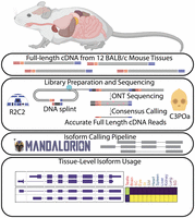
Experimental overview. Full-length cDNA was created from total RNA extracted from 12 BALB/c mouse tissues. Pooled cDNA, both non-size-selected and size-selected (see text), was prepared for ONT sequencing by the R2C2 method. ONT raw reads were demultiplexed and consensus called using C3POa which identifies and combines low-accuracy subreads to create high-accuracy consensus reads. To generate a tissue-level transcriptome for each tissue, R2C2 consensus reads were then processed into isoforms using the Mandalorion pipeline. (SC) spinal cord, (St) stomach, (SM) skeletal muscle, (SG) salivary gland.
We then prepared non-size-selected (nss) and size-selected (ss) full-length cDNA for ONT sequencing using the R2C2 protocol.
Because the LRGASP effort had shown that preparing and sequencing R2C2 DNA can introduce different biases between batches (Pardo-Palacios et al. 2024b), we aimed to minimize these batch effects. To do so, we pooled DNA from all samples before preparing it for sequencing (see Methods). In addition to minimizing batch effects, pooling samples also streamlined sample preparation and sequencing. Further, because every sample was present in each sequencing library at approximately the same ratio we could sequence our sample pools across many ONT flow cells—both on the MinION and PromethION—and combine the resulting data, all while generating very similar read numbers for each sample.
We sequenced the resulting, pooled DNA using R9.4 pore chemistry and SQK-LSK110 library preparation kits. After basecalling the raw signal data using Guppy (v5) (Wick et al. 2019), we generated accurate full-length cDNA consensus reads using the C3POa pipeline (Volden et al. 2018), which also demultiplexed the resulting consensus reads into their tissue of origin. In this way, we produced 64 million full-length cDNA consensus reads, averaging 5.4 million reads per tissue (Fig. 2, top). For nss libraries, the median insert length was ∼750 bp while the ss libraries had a median insert length ∼2 kb (Fig. 2, center). Further, the full-length R2C2 consensus reads were very accurate, with the median per base identity for nss and ss reads being 99.8% and 98.9%, respectively (Fig. 2, bottom). The lower accuracy of the ss reads was due to longer cDNA inserts being covered less often by ONT raw reads.
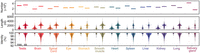
R2C2 read characteristics. (Top) Read counts in millions split between nss and ss libraries. (Center) Insert length split between nss and ss libraries. (Bottom) Read accuracy of C3POa full-length consensus reads split between nss and ss libraries.
Evaluating gene-level expression quantification
Next, we investigated whether the full-length cDNA R2C2 reads we generated could be used for gene detection and expression quantification. To this end, we compared the R2C2 data set to publicly available Illumina RNA-seq data generated for different samples of the same 12 tissues (Brawand et al. 2011; Mustafi et al. 2011; Merkin et al. 2012; O'Rourke et al. 2015; Gluck et al. 2016; Huntley et al. 2016; Söllner et al. 2017), and data available at the NCBI Sequence Read Archive (SRA; https://www.ncbi.nlm.nih.gov/sra) under accession SRR2927121. First, we aligned R2C2 and Illumina RNA-seq reads to the GRCm39 mouse reference genome sequence using minimap2 (Li 2018) and STAR (Dobin et al. 2013) aligners, respectively. While minimap2 does not use a genome annotation to aid alignment, STAR used the GENCODE vM30 annotation. We then quantified gene expression based on both R2C2 and Illumina RNA-seq alignments using featureCounts (Liao et al. 2014) and the GENCODE vM30 annotation. By default, featureCounts counts the number of reads that overlap with each gene in the annotation by at least one base pair and ignores reads that overlap with more than one gene.
The first analysis we performed aimed to determine if our R2C2 sequencing depth was enough to detect all genes expressed in the samples. To perform saturation analysis, we subsampled both R2C2 and Illumina RNA-seq data. We counted genes as detected if featureCounts assigned them at least one read in the subsampled Illumina and R2C2 data sets. We saw the R2C2 data set approaching a plateau but with fewer total genes detected than the Illumina data (Fig. 3A,B). This can be attributed to the almost 10-fold difference in read counts, but also the fact that, in contrast to full-length cDNA sequencing, fragmentation-based short-read Illumina RNA-seq can detect genes entirely independently of their length.
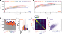
R2C2 and Illumina RNA-seq detect largely the same genes at similar levels. Gene-level saturation curve analysis of R2C2 data (A) and Illumina RNA-seq data (B). (C) Comparison of genes detected by either R2C2 or Illumina RNA-seq or both. (D) Expression levels as determined by R2C2 and Illumina RNA-seq for genes detected by either R2C2 or Illumina RNA-seq or both (colors as in A). (E) Pearson's correlation between gene expression values was determined by R2C2 and RNA-seq for each tissue. (F) Scatterplot of kidney gene expression values as determined by R2C2 and Illumina RNA-seq. (SC) spinal cord, (St) stomach, (SM) skeletal muscle, (SG) salivary gland.
Next, we compared the genes detected by the full R2C2 and Illumina RNA-seq data sets. Across all tissues, Illumina RNA-seq detected more genes than R2C2 (Supplemental Table S1). For each tissue, we then determined the number of genes detected by either R2C2 only, Illumina RNA-seq only, or both methods (Fig. 3C). The majority of genes detected were identified by both methods and more genes were identified by Illumina RNA-seq only than R2C2 only. However, the genes that were identified by only one of the two methods were generally expressed at very low levels (Fig. 3D). This also explains why genes might be missed by either method and also why Illumina RNA-seq with its higher read count might detect more genes than R2C2 (Fig. 3D).
In addition to detecting genes, we analyzed whether R2C2 was quantitative in determining their expression. We did so by again using featureCounts output for each analyzed tissue. After converting the raw read counts determined by featureCounts to reads per million (RPM), we compared R2C2-derived to Illumina RNA-seq-derived gene expression for each tissue. We found that R2C2 gene expression was most correlated to Illumina RNA-seq gene expression for the same tissue with Pearson r value ranging from somewhat correlated (Spleen r = 0.22) to well correlated (Lung r = 0.78) (Fig. 3E,F; Supplemental Table S2). Neuronal tissues (brain, spinal cord, eye) also showed a high correlation between tissues.
The lower correlation between R2C2 and Illumina RNA-seq in some tissues could be due to biological differences between the RNA samples we used and those underlying the publicly available Illumina data, like the overall health status of the animal, or, most importantly, what part of the tissue was sampled. These differences highlighted the limitation of using publicly available data. Generally, the gene overlap and high expression correlation between R2C2 and Illumina data in at least some tissues suggest that combining R2C2 data from ss and nss cDNA does not substantially distort gene content and expression.
Characterizing tissue-level isoforms
To take full advantage of our long-read data, we aimed to use the full-length R2C2 consensus reads to move beyond gene-level analysis and define comprehensive sets of isoforms for each of the 12 tissues in this study. To identify isoforms in a way that has high Recall and Specificity, especially with unannotated isoforms, we analyzed the R2C2 reads we produced using the Mandalorion (v4.0) tool (Volden et al. 2023; Pardo-Palacios et al. 2024b). Mandalorion identifies, filters, and quantifies isoforms to create high-confidence sets of transcript isoforms and was identified by the LRGASP effort to have a good balance of sensitivity and precision (Pardo-Palacios et al. 2024b).
For the individual tissue data sets, Mandalorion identified between 22,727 (salivary gland) and 63,948 (testis) isoforms (Supplemental Table S3). To investigate whether we sequenced these transcriptomes to exhaustion, i.e., more reads would not result in more isoforms being identified, we performed a saturation analysis for each tissue (Fig. 4A). We did not reach saturation for any tissue which meant our transcriptome annotations are not exhaustive and are likely to miss many low abundance transcripts.
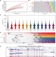
Characterization of tissue-level transcriptomes. (A) Isoform saturation curves for each tissue. (B) Isoform category distributions for each tissue as determined by SQANTI3 (full splice match [FSM], novel in catalog [NIC], novel not in catalog [NNC], incomplete splice match [ISM], intergenic [IG], antisense [AS]). (C) Isoform length distribution for each tissue compared to GENCODE vM30 basic protein-coding transcripts. (D) For each tissue, genes are rank-ordered based on their expression level in Illumina RNA-seq data. Genes are marked by a vertical colored line if at least a single isoform is assigned to them in the respective tissue; 0, 1, and 5 RPM levels in RNA-seq data are indicated by black lines. The percentage of genes expressed higher than that RPM with at least one isoform assigned to them is shown adjacent to those lines. (E) Screenshot of the testis, spleen, and kidney tracks from the TAMI trackhub as displayed on the UCSC Genome Browser.
Next, we wanted to compare the isoforms we identified to the 149,419 isoforms transcribed from 56,691 genes (21,668 of them protein-coding) present in the GENCODE vM30 annotation. For this comparison, we used SQANTI3 (Tardaguila et al. 2018; Pardo-Palacios et al. 2024a) which assigns experimentally identified isoforms to annotated isoforms and genes and further classifies them. On average, ∼2 isoforms each were assigned to between 12,023 (salivary gland) and 26,784 (testis) genes (Supplemental Table S3). Between 61% (testis) and 88% (lung) of these genes were present in the GENCODE annotation (Supplemental Table S3). Across all tissues, an average of 91% of these annotated genes were classified as the gene type “protein_coding” by GENCODE, followed by “lncRNA” (7%) and “processed_pseudogene” (1%) (Supplemental Table S4).
For each tissue, SQANTI3 further categorized each Mandalorion isoform based on how their splice sites and junctions compare to annotated isoforms in the GENCODE vM30 annotation reference file (Fig. 4B).
The four main categories SQANTI3 uses are “full splice match” (FSM), “incomplete splice match” (ISM), “novel in catalog” (NIC), and “novel not in catalog” (NNC). If the set of splice junctions present in a Mandalorion isoform is identical to all splice junctions present in an annotated reference isoform, the Mandalorion isoform is categorized as a “FSM”. Importantly, the 5′ and 3′ ends of the FSM isoforms do not have to match those of their annotated reference isoform. If the set of splice junctions present in a Mandalorion isoform is a continuous but incomplete subset of splice junctions present in an annotated isoform, the Mandalorion isoform is categorized as an “ISM”. If all splice sites present in a Mandalorion isoform are present in any annotated isoform, the Mandalorion isoform is categorized as “NIC”. If at least one splice site present in a Mandalorion isoform is not present in any annotated isoform, the Mandalorion isoform is categorized as “NNC”.
There are additional SQANTI3 categories, like “intergenic” (IG), “antisense” (AS), “genic intron,” and “genic genomic,” describing isoforms falling outside of genes, on the opposite strand of a gene, within intron, or within introns and exons, respectively.
However, across tissues, we see ∼80%–90% of isoforms falling into the four main categories at similar rates (average FSM 54%, NIC 16%, NNC 6%, ISM 8%), with the exception of the testis which showed a higher number of NNC isoforms indicating the use of many unannotated splice junctions (Fig. 4B; Supplemental Table S5).
Across tissues, isoforms were ∼2 kb in median length with the exception of the testis which contained shorter isoforms overall (Fig. 4C). The isoforms we identified were, therefore, shorter than the protein-coding transcript isoforms present in GENCODE. In particular, due to R2C2 read length limitations, the isoforms we identified lacked the long tail >6 kb of isoforms present in GENCODE annotations, which represented 7.5% and 17.7% of all and protein-coding GENCODE transcript, respectively.
Although missing low-expressed and very long isoforms, we wanted to check whether the isoform-level genome annotations we generated would still represent valuable resources by at least containing the major isoforms for many expressed genes. We, therefore, quantified the percentage of genes expressed in the Illumina RNA-seq data for which we identified at least one isoform. We found that, on average across tissues, Mandalorion identified at least one isoform for ∼75% and ∼86% of genes with >1 RPM and 5 RPM expression levels in the Illumina RNA-seq data, respectively (Fig. 4D).
In summary, we generated isoform-level genome annotations which are likely to lack low abundance and very long isoforms. These genome annotations contained tens of thousands of new, high-confidence isoforms (NIC, NNC). Finally, they contained at least one isoform for the majority of medium to highly expressed genes which should make them a valuable resource for molecular biology research and experimental design.
Tissue-level Atlas of Mouse Isoforms
To make this resource as easily accessible for researchers as possible, we have created a trackhub for the UCSC Genome Browser (Navarro Gonzalez et al. 2021). Entitled TAMI, this trackhub is available at https://genome.ucsc.edu/s/vollmers/TAMI for the GRCm39 (GCA_000001635.9) version of the mouse genome. TAMI contains separate tracks for each tissue (Fig. 4E) which contain isoform models identified by Mandalorion for that tissue. Isoform expression levels are normalized within each gene and that normalized expression is then shown by the color of each isoform. Absolute expression in RPM can be seen by positioning the cursor over an isoform. An alignment between the R2C2 read-based consensus sequence of each isoform and the corresponding genomic sequence is available by clicking the isoform. These alignments might highlight potential sequencing errors as well as variation between the BALB/c isoforms and the GRCm39 genome which is based on the C57BL/6 strain. Overall, the goal of the TAMI track is to give researchers fast and intuitive information about their genes of interest.
Investigating unique TSS usage in testis
When creating and inspecting the TAMI tracks for release, we observed that, often, isoforms expressed in testis would use unique, testis-only TSSs. This made sense considering testis is known to be the most transcriptionally complex tissue in mammals in terms of the number of expressed genes and isoforms (Kaessmann 2010).
The systematic analysis confirmed this unique TSS usage. We found that the 63,948 isoforms expressed in testis originated from 31,158 nonoverlapping TSSs. Of those, 16,522 were unique to testis. This number of unique, tissue-restricted TSSs in the testis was much higher than any of the other tissues we investigated (Fig. 5, top).
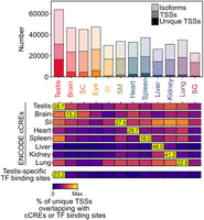
Unique TSSs in testis are bound by testis-specific transcription factors. (Top) Number of isoforms, overall TSSs, and TSSs unique to a tissue are shown for each tissue. (Bottom) Heatmap of the percent of unique TSSs of each tissue overlapping with ENCODE cCREs of the indicated tissues or with testis-specific transcription factor binding sites. Each row represents an individual heatmap normalized between 0 and the maximum for that row (shown as text within each row). Therefore, color intensity cannot be compared between different rows. (SC) spinal cord, (St) stomach, (SM) skeletal muscle, (SG) salivary gland, (SI) small intestine.
First, we wanted to validate these unique tissue-restricted TSSs using candidate cis-regulatory elements by ENCODE (cCREs) (The ENCODE Project Consortium et al. 2020). These cCREs were determined using a mix of ChIP-seq, ATAC-seq, and DNA-seq, and included regulatory features like potential promoters. For analysis, we downloaded these cCREs for eight tissues (testis, brain, small intestine [equivalent to smooth muscle], heart, spleen, liver, kidney, and lung) that matched tissues we analyzed for TAMI. We then evaluated the percentage of unique TSSs of each tissue that overlapped with these cCREs. We found that a higher percentage of unique TSSs of a specific tissue overlapped with cCREs of that specific tissue than the unique TSSs of the other 11 tissues (Fig. 5, bottom). This showed that the unique tissue-restricted TSSs we identified based on isoforms matched candidate regulatory elements of their respective tissues, which in turn were identified with an entirely different set of methods by ENCODE.
Second, we wanted to validate the unique TSSs of the testis with transcription factor ChIP-seq data from ChIP-Atlas (https://chip-atlas.org) (Oki et al. 2018). First, we evaluated the expression patterns of the transcription factors that had been investigated in testis (Supplemental Fig. S1, left). We found that, based on our R2C2 data, several of these transcription factors were indeed most highly expressed in testis. The binding sites of these testis-specific transcription factors, as determined by many distinct ChIP experiments, were generally enriched in TSS unique to the testis (Supplemental Fig. S1, right).
Based on this analysis, we selected a single ChIP-seq experiment for just six testis-specific transcription factors—TAF7L, TCFL5, SOX30, MYBL1, RFX2, TBPL1 (Zhou et al. 2013, 2017; Kistler et al. 2015; Martianov et al. 2016; Yin et al. 2021; Cecchini et al. 2023). We found that 23% of unique testis TSSs but only ∼3% of the unique TSSs of the other tissues overlapped with their combined binding sites (Fig. 5, bottom).
This indicated that, within the testis, testis-specific transcription factors create isoform diversity through the use of unique TSSs. The high percentage of NNC isoforms in testis suggests that those unique TSS are often unannotated.
Differential isoform usage across tissues
The quantitative nature of the R2C2 approach as well as the multiplexed setup of our sequencing strategy allowed us to compare isoform expression across tissues. To avoid the complexity of merging 12 individual annotations, we used Mandalorion to identify isoforms from the combined data set of all 12 tissues and to quantify the expression of those isoforms in each tissue.
First, we evaluated which tissues were expressing the same isoforms—at any level—by calculating Jaccard indexes for each pair of tissues (Fig. 6A). Again, testis proved an outlier, having lower Jaccard indexes, i.e., the smallest overlap of isoforms, than any other tissue. As expected, neuronal tissues (brain, spinal cord, and eye) had high Jaccard indexes with each other. The stomach and smooth muscle (small intestine), both parts of the digestive system, also had a high Jaccard index.
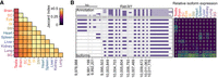
Differential isoform usage. (A) Jaccard indexes for each pair of tissues, (B) Genome Browser shot of Rab3il1 is shown with GENCODE vM30 annotation on top and isoforms called by Mandalorion below. Right side, the relative usage of each isoform in each tissue, yellow indicates higher usage, blue indicates lower usage. (SC) spinal cord, (St) stomach, (SM) skeletal muscle, (SG) salivary gland.
Second, to systematically identify genes with differential isoform expression across tissues, we first identified 7457 genes that had a combined isoform expression of at least 50 R2C2 reads (∼10 RPM) in at least two tissues. We then performed a χ2 contingency table test on the relative isoform usage of each of those genes. After Bonferroni correction, we found 3742 genes with significant differential isoform usage at P ≤ 0.01. An example of one such gene, Rab3il1 shown in Figure 6, highlights differential isoform usage across tissues particularly in regards to the use of alternative TSS and first exons, as well as alternative internal exon usage within the same tissue.
Overall, our analysis shows if a gene is expressed moderately high in at least two tissues, it is more likely than not (3742 out of 7457 or ≈50.2%) to show differential isoform expression.
Discussion
Here, we have presented a genome annotation atlas for the mouse, highlighting the immense isoform diversity between different tissues. We used the ONT-based R2C2 method to sequence over 60 million full-length transcripts across 12 tissues. We compiled these reads using the Mandalorion tool (Volden et al. 2023; Pardo-Palacios et al. 2024b) and the resulting isoforms formed the basis for the first release of the TAMI which is hosted as a trackhub on the UCSC Genome Browser.
We hope these tracks and their source files will be a valuable resource for genomics research by, for example, complementing existing annotations with tissue-specific information for transcriptome-dependent RNA-seq analysis by tools like Salmon (Patro et al. 2017) and kallisto (Bray et al. 2016). Further, by identifying more accurate transcript ends, TAMI might improve the analysis of scRNA-seq data whose reads are most often limited to the 3′ or 5′ end of transcripts.
We also hope that TAMI will be of value to bench scientists by providing easy-to-access detailed isoform information and thereby informing experimental design. For example, instead of cloning a random isoform taken from GENCODE or RefSeq for overexpression, TAMI enables you to clone the isoform that is most expressed by your gene of interest in your tissue of interest.
TAMI v1.0 represents only a starting point for our annotation efforts because it is limited in certain important ways. First, TAMI v1.0 only includes 12 major tissues which leaves many tissues and cell types unannotated. Further, the read numbers TAMI v1.0 is based on are too low to exhaustively cover the transcriptome of those 12 tissues often limiting it to the major isoforms of genes. Additionally, despite size selection, these reads are too short to capture the longest mouse transcripts effectively. Finally, TAMI v1.0 still relies on ONT R9 chemistry, which has been replaced by the more accurate R10 chemistry.
To address these shortcomings, we plan on using updated technologies and methods including the PacBio Kinnex method, automated cDNA size selection, and ONT R10 pores to generate more, longer, and more accurate full-length cDNA reads for a larger number of tissues and cell types. In preparation for these data sets, we have also recently rewritten the Mandalorion (Volden et al. 2023) tool to be capable of handling the much larger >100 million full-length cDNA read data sets that are now becoming a reality. For the next version of TAMI, we are also working using tools like IsoAnnotLite to predict open reading frames for protein-coding isoforms.
This will be an important follow-up because we found widespread isoform diversity between tissues. Investigating how and whether this isoform diversity between tissues creates biological meaningful differences in the function of genes in these tissues will benefit from the information on whether different isoforms of a given gene encode different proteins.
We will also continue work to improve and validate gene and transcript level quantification. In this study, we compared R2C2 full-length cDNA sequencing-based gene-level quantification to quantification based on publicly available Illumina RNA-seq data and found that the methods detected overlapping but distinct sets of genes, with Illumina RNA-seq detecting more genes overall. We also found that gene-level expression quantification had sometimes low correlation between R2C2 full-length cDNA sequencing and Illumina RNA-seq. To remove biological variability from this comparison in the future, we will generate deeply sequenced Illumina RNA-seq data sets on the same RNA samples used for R2C2 full-length cDNA sequencing going forward.
Other limitations of TAMI v1.0 that we will not be able to address are rooted in the reliance of the Smart-seq2-based cDNA synthesis approach on oligo(dT) primers and size selection. While this effectively excludes ribosomal RNA, it also excludes many other species of RNA that are either short, not poly-adenylated, or both which includes histone RNA and many short noncoding RNA species like tRNA.
Another potential concern associated with TAMI is that we analyzed the data we generated using Mandalorion, a tool we developed and maintained over the last 7 years, as opposed to other isoform identification and quantification tools. While Mandalorion has been shown by the LRGASP consortium and our own manuscript to display a strong balance between Specificity and Recall—especially when identifying previously unannotated isoforms—other tools like IsoQuant have done so as well (Prjibelski et al. 2022; Volden et al. 2023; Pardo-Palacios et al. 2024b). Indeed, when we reanalyzed all the data in TAMI with IsoQuant, the resulting isoform sets for each tissue were similar to the corresponding Mandalorion sets (Supplemental Fig. S2A, left). IsoQuant also identified testis as an outlier tissue in terms of isoform composition (Supplemental Fig. S2A, center, right). Additional analysis by SQANTI3 showed that the different tools produced similar compositions of structural isoform categories (FSM, NIC, …) with Mandalorion producing more FSM and IsoQuant producing more NNC isoforms (Supplemental Fig. S2B).
Beyond that, however, our comparison showed known behavior of IsoQuant that made it unsuited for this study. First, if IsoQuant identifies an isoform that matches an isoform in the reference (FSM isoforms), it reports the TSS and transcription termination site (TTS) of the reference isoform (Supplemental Fig. S2C). This means that the ends of IsoQuant FSM isoforms (which comprise ∼50% of all isoforms in the study), in contrast to Mandalorion FSM isoforms, do not reflect the actual reads present in the sample and, therefore, might not reflect the actual biology of the sample. Further, even for the other categories, IsoQuant isoforms had lower CAGE peak support, i.e., support by an experimentally determined TSS, than Mandalorion isoforms (Supplemental Fig. S2D). While this is indirect evidence, it nonetheless indicates that Mandalorion isoforms have ends that better reflect the actual TSSs of the isoforms expressed within a sample. Because TSSs in particular are very important for downstream experiments (locating the exact promoter, proper 5′UTR, and correct CDS) Mandalorion was clearly the better choice for our study. However, we contend that there are now many other isoform identification tools that due to their design choices might uncover unique features of the TAMI data set.
Finally, while TAMI is intended to merely complement the excellent manually curated reference annotations like GENCODE that are available for mouse, this paper shows that, going forward, full-length cDNA-based annotation efforts could serve as reference annotations for less researched organisms.
We think TAMI provides a blueprint for these efforts. The generation of indexed cDNA makes it possible to pool samples early which in turn allows for the cost-effective generation of sequencing libraries. ONT sequencing, due to its low device cost, can be performed in most molecular biology labs. Finally, data analysis, including Mandalorion-based isoform identification, can be performed on consumer-grade computers. All of this puts genome annotation efforts within reach of individual laboratories with moderate budgets.
Methods
Sample multiplexing
RNA was acquired from Takara Bio (Cat# 636644). Multiplexing samples was done using one of two methods: the first used barcoded DNA splints for Gibson assembly then pooling samples after rolling circle amplification (RCA), and the second method used barcoded oligo(dT) for cDNA synthesis which allowed pooling before Gibson assembly. Both methods produce equivalent data. Approximately 80% of the data used in this study was generated by using barcoded oligo(dT) primers for multiplexing tissues.
Library preparation and sequencing
cDNA synthesis
RNA was first mixed with dNTPs and oligo(dT) primer, either barcoded or nonbarcoded, then denatured to remove the secondary structure for 3 min at 72°C. First strand reverse transcription (RT) using SMARTScribe Reverse Transcriptase (Clontech) and Smart-seq2 template switching oligo (TSO) with DTT and SUPERaseIN was performed for 1 h at 42°C then heat inactivated for 5 min at 70°C. Second strand synthesis and PCR with KAPA 2× master mix and ISPCR primer with RNase A and lambda exonuclease for 12 cycles (37°C for 30 min, 95°C for 3 min, 98°C for 20 sec, 67°C for 15 sec, 72°C for 8 min, 72°C for 5 min, 4°C hold). cDNA was cleaned up and ss using SPRI beads at a 1:0.85 (sample:beads). After quantification by Qubit the cDNA libraries were pooled together if barcoded oligo(dT) primers were used, if not, cDNA from individual tissues would still be kept separate. The cDNA was then split for ss and nss R2C2 library preparation. For size selection, cDNA was run on a 1% low melt agarose gel and everything over 2 kb was excised and purified using beta-Agarase digestion and SPRI bead clean up.
R2C2 library generation
ss and nss cDNA were further processed separately but identically. cDNA libraries were circularized by Gibson assembly (NEBuilder HiFi) with a short DNA split that overlaps with the ends of the cDNA. For cDNA that was not barcoded during cDNA synthesis a barcoded DNA split was used. To remove uncircularized molecules, an exonuclease digestion with ExoI, ExoII, and Lambda Exonuclease (all NEB) was carried out for 16 h at 37°C then heat inactivated for 20 min at 80°C. The reaction was then cleaned using SPRI beads at a 1:0.85. The clean, circularized library is then used as a template for RCA using Phi29 (NEB) with a random hexamer primer for 18 h at 30°C then heat inactivated for 10 min at 65°C. The Phi29 reaction was then debranched using T7 endonuclease for 2 h at 37°C before being cleaned and concentrated using Zymo DNA clean and concentrator column. The library was quantified by Qubit and gel extracted as described above but the region extracted was a bright band just over the 10 kb marker. After gel extraction, the library was quantified again by Qubit.
ONT sequencing
Libraries barcoded during the Gibson assembly step were now pooled together at equal mass. We used the Ligation Sequencing Kit for genomic DNA (SQK-LS110) from ONT to prepare for sequencing following the manufacturer's protocol. The final library was loaded onto either an ONT MinION or PromethION sequencer. Flowcells were nuclease flushed and loaded with additional library partway through sequencing based on pore availability statistics shown in the MinKNOW software to increase sequencing throughput.
Data processing
All ONT FAST5 files were basecalled using Guppy (v5) (Wick et al. 2019) with the super accurate configuration. R2C2 full-length consensus reads were generated and demultiplexed by C3POa (v2.4.0).
Analysis
Gene-level analysis
R2C2 reads were aligned to the GRCm39 version of the mouse genome using minimap2 (v2.24-r1122) (Li 2018) with the following arguments. -ax splice ‐‐secondary=no. Read accuracy was calculated by identifying mismatches and indels in those alignments.
Illumina reads were aligned using STAR aligner (v2.5.4b) (Dobin et al. 2013) to a genome index built with the same version of the genome and the GENCODE vM30 comprehensive annotation with the following arguments:
‐‐outSAMattributes NH HI NM MD AS nM jM jI XS ‐‐quantMode GeneCounts.
For both R2C2 and Illumina data, gene-level expression was quantified based on these aligned reads using featureCounts (v1.6.0). The resulting counts were converted to RPM by dividing the number of reads associated with each gene by the total number of reads then multiplying by 1 million. Pearson's correlation comparing Illumina and R2C2 gene quantification were produced using non-log-converted RPM featureCounts.
Gene-level saturation curves were produced by random subsampling of the featureCounts output for each tissue and the combined data set.
Isoform-level analysis
Isoforms were called based on R2C2 reads using the Mandalorion Isoform analysis pipeline (v4.0) run on both individual tissue data and the combined data set using defaults settings and the GENCODE vM30 annotation and GRCm39 reference sequence. Mandalorion isoforms were produced from both individual tissues and the combined data set. The resulting isoforms were categorized and compared to the GENCODE vM30 annotation using the sqanti_qc.py script of SQANTI3 v5.1 (Pardo-Palacios et al. 2024a).
Isoform-level saturation curves were produced by random subsampling R2C2 reads and running Mandalorion (Volden et al. 2023) independently for each subsample. Differential isoform usage analysis was performed on the isoforms from the combined data set using the χ2 contingency test with a custom Python script utilizing SciPy (Supplemental Code; Jones et al. n.d.; Harris et al. 2020).
Jaccard index
To compare isoform compositions of different tissues, we calculated Jaccard indexes for each pair of tissues. We used the isoforms and their expression levels from the combined data set. Isoforms were counted as present in a tissue if they had at least one read associated with them in that tissue. We then calculated the Jaccard index as follows: ([Isoforms shared between tissues A and B]/[Isoforms shared between tissues A and B + Isoforms unique to tissue A + Isoforms unique to tissue B]).
To compare isoform compositions between Mandalorion and IsoQuant, we first compiled the gtfs from each tissue and tool using gffcompare (v0.12.6.OSX_x86_64) (Pertea and Pertea 2020). We then parsed gffcompare output to determine shared and unique isoforms for each pair of tissues/tools and calculated Jaccard indexes as above.
TSS level analysis
A tissue-unique TSS was determined by first combining TSS that were <100 nt apart within each tissue and then comparing the combined TSSs of each tissue to all other tissues. A tissue-unique TSS was defined as a TSS in one tissue that does not overlap with TSSs in any other tissue.
cCRE analysis
cCREs for testis, brain, small intestine (equivalent to smooth muscle), heart, spleen, liver, kidney, and lung were downloaded from SCREEN: Search candidate cis-regulatory elements by ENCODE (Registry of cCREs V3). The resulting tissue-specific BED files all contained all cCRE locations in the entire data set. cCRE annotated to be functional in each respective tissue were filtered from these BED files and overlapped with the unique TSSs of each tissue in the study.
ChIP-atlas-based testis TF analysis
A custom Python script was used to determine TSS overlaps with publicly available ChIP-seq (https://chip-atlas.org, accessed in Spring 2023) (Supplemental Code). Data from ChIP-Atlas were downloaded as a BED file from the peak browser tool by selecting the following options: Assembly: M. musculus mm10, experiment type: ChIP TF, Cell Type Class: Gonads, Threshold for Significance: 50, ChIP Antigen: all, Cell Type: testis.
IsoQuant comparison
To compare isoform compositions of different tissues and tools, we calculated Jaccard indexes for pairs of isoform sets. To make the isoform sets comparable in principle, we applied a minimum cutoff of three reads per isoform and excluded all single-exon isoforms from all IsoQuant and Mandalorion isoform sets. We used gffcompare to compare the 24 filtered isoform sets (12 tissues × 2 tools). We then parsed the gffcompare output and calculated the Jaccard index as follows: ([Isoforms shared between tissues A and B]/[Isoforms shared between tissues A and B + Isoforms unique to tissue A + Isoforms unique to tissue B]).
Data access
The full-length consensus reads generated in this study have been submitted to the NCBI BioProject database (https://www.ncbi.nlm.nih.gov/bioproject/) under accession number PRJNA971991. Isoform models in GTF format generated in this study are hosted and updated at https://vollmerslab.sites.ucsc.edu/tami and also available as Supplemental Data.
Competing interest statement
The authors declare no competing interests.
Acknowledgments
The ONT Promethion sequencing was carried out by the DNA Technologies and Expression Analysis Core at the UC Davis Genome Center, supported by the National Institutes of Health (NIH) Shared Instrumentation Grant 1S10OD010786-01. This work was supported by the NIH R35GM133569 to C.V.
Author contributions: M.A. and C.V. conceived of the study; M.A. performed experiments, analyzed and visualized data, and wrote the first draft of the manuscript; C.V. secured funding for the research, analyzed and visualized data, and edited the manuscript.
Footnotes
-
[Supplemental material is available for this article.]
-
Article published online before print. Article, supplemental material, and publication date are at https://www.genome.org/cgi/doi/10.1101/gr.279217.124.
-
Freely available online through the Genome Research Open Access option.
- Received February 29, 2024.
- Accepted September 11, 2024.
This article, published in Genome Research, is available under a Creative Commons License (Attribution-NonCommercial 4.0 International), as described at http://creativecommons.org/licenses/by-nc/4.0/.


