Panel of Microsatellite Markers for Whole-Genome Scans and Radiation Hybrid Mapping and a Mouse Family Tree

Leonard C. Schalkwyk; Martin Jung; Angelika Daser; Michael Weiher; Jörn Walter; Heinz Himmelbauer; Hans Lehrach

doi:10.1101/gr.9.9.878

Abstract

To facilitate whole-genome scan experiments, we selected a panel of 128 microsatellite markers on the basis of spacing and polymorphism in the strains DBA/2, BALB/c, AKR, C57BL/6, C57BL/10, A/J, C3H, 129/J, SJL/J, JF1, and PWB. Many of the primer pairs were redesigned for better performance. The last four strains were not characterized previously using these markers. JF1 and PWB are particularly interesting for intersubspecific crosses offering high polymorphism. We provide allele size data for the markers on these strains and add them to the emerging radiation hybrid framework map, which is not continuous except for chromosome 17 and 13. Information on the interrelationships of strains is useful both because of the importance of polymorphism in designing crosses and the background in assessing phenotypes. Microsatellites offer a widely dispersed, selectively neutral set of characters that lends itself conceptually to parsimony methods of analysis. The microsatellite allele size data were recoded as binary discrete characters in such a way that adjacent sizes differ by one step. Trees were generated using a Wagner parsimony method. As expected, the non-Mus domesticus strains, PWB (musculus) and JF1 (molossinus), are excluded from the domesticus strains. Among the domesticus strains, C57BL/6 and C57BL/10 (derived from the same founding pair) form a strongly supported group, as do C3H, A/J, and BALB/c (derived from the Bagg albino stock). No unique branching order for SJL/J, AKR, and DBA/2 is strongly supported, which may reflect a complicated history. Strain 129/J is clearly placed as the most deeply diverged of thedomesticus strains represented.

To map quantitative trait loci it is necessary to test the genotypes of cross progeny with a panel of polymorphic markers spaced at 10- to 20-cM intervals. For example, with 52 backcross animals, linkage across 15 cM can be detected at 95% confidence. Therefore, in principle, a set of markers no more than 15 cM from chromosome ends and 30 cM from each other would suffice (Silver 1995). Although there are now many microsatellite markers available (primarily MIT markers from Dietrich et al. 1996) and the average density is about four markers/cM, it is still often difficult to find sufficient markers with differing alleles for a particular pair of inbred strains. This is especially true if these are both derived fromMus musculus domesticus. In addition, although the quality of published microsatellite markers is good, most of them are mass-produced and have not been extensively characterized, and some primers are not robust. For the Dietrich et al. (1996) markers, allele size data are available for 12 strains, including a Mus spretus and a Mus musculus castaneus strain. However, for any given pair of strains it is a substantial job to identify a suitable marker panel and verify that these are detectably polymorphic.

We have selected a set of highly polymorphic markers for the Mus musculus strains DBA/2, BALB/c, AKR, C57BL/6, A/J, and C3H (typed by Dietrich et al. 1996), redesigned many of the primers, and tested them on these strains, as well as C57BL/10, SJL/J, 129/J, JF1, and PWB. PWB is an inbred strain derived from a wild-derived Czech Mus musculus musculus isolate (Forejt 1991). JF1 is a recently established inbred strain of Japanese Mus musculus molossinusorigin (a natural hybrid of M. m. musculus and M. m. castaneus; Bonhomme and Guénet 1996), which should also differ at many loci from the standard strains (Koide et al. 1998). The remaining strains are classic inbred strains that are quite closely related (Silver 1995). 129/J in particular is a widely used strain for which allele size data are not provided in the MIT data set. Data for 209 simple sequence-length polymorphisms (SSLPs) on strain 129 were published recently (Matin et al. 1998), only 2 of which are in common with the work reported here.

It would be useful to have a clear picture of the degrees of relatedness of mouse strains to each other. The breeding histories of the classical inbred strains are to some extent known (Festing 1996), but there are little data on the outbred progenitor populations. The relationships of the inbred strains of mice were investigated using parsimony by Atchley and Fitch (1991), employing classical genotypes at 144 loci over the whole genome. At each locus, possession by two strains of the same-sized allele indicates probable similarity by descent of that sequence. Using many loci spread over the genome, it should be possible to reconstruct a phylogeny of the genome as a whole, at least to the extent that the history of these strains can be represented by a tree (i.e., no recent interbreeding, which would give a net). Atchley and Fitch (1991) obtained a tree that reflected the groups of strains known to be closely related: the C57 and C58 strains, and the Bagg albino descendants BALB/c, A, and C3H. A somewhat deeper clade united many of the others, including SJL, DBA, and AKR. The main findings were reproduced by a subset of the data identified as “protein loci” but not by smaller subsets of “immune” and “viral.” One discrepancy between the overall and protein trees is the position of strain 129, which is a specific relative of the C57 and C58 group in the former and of the SJL/DBA/AKR group in the latter.

Radiation hybrid (RH) panels are an attractive tool for mapping arbitrary sequences (such as ESTs) without the need for polymorphism and high resolution, and have been important in making a very gene-rich human map (Deloukas et al. 1998). The T31 panel has been characterized sufficiently to indicate that it will be a useful mapping tool. Typings of 472 markers on the panel are available from the public database (http://www.jax.org/resources/documents/cmdata/rhmap/rhdata.html). This database includes the initial characterization (McCarthy et al. 1997) and detailed maps of chromosome 17 (Schalkwyk et al. 1998) and chromosome 13 (Elliott et al. 1999). However, these data do not provide a framework suitably dense to allow unknown markers to be mapped with certainty. We have typed the T31 RH panel (McCarthy et al. 1997) with the same panel of markers and thus contributed to an emerging map framework for this panel.

RESULTS AND DISCUSSION

The panel of microsatellite markers was selected using published genetic positions and allele sizes (Breen et al. 1994; Dietrich et al. 1996) with two objectives: maximizing polymorphism in our chosen list of strains, and approximating a 10-cM spacing. This resulted in a preliminary list of 148 markers, 114 of which were selected. The remaining markers did not produce the expected PCR performance, polymorphism, or position. Another 14 markers were selected to patch the resulting gaps. Primer sequences were inspected for potential problems and redesigned where possible to eliminate cases where the 3′ end contained one or more CA dinucleotide sequences, which experience indicates leads to stuttering artifacts. Other primer sequences were redesigned to adjust the sizes of the products to facilitate multiplexing of the markers within chromosomes.

Mouse Strain Panel Data

The 11 strains tested here (allele size data presented in Table1) give rise to 55 pairs of strains that could be considered for a cross. For different pairs, the present work provides between 31 and 120 polymorphic markers (Table 2)—in many cases, a nearly complete, tested panel of markers. The allele size data, as well as lists of polymorphic markers for each possible pair, are available athttp://www.mpimg-berlin-dahlem.mpg.de/∼rodent/bin/polymarkerleo.cgi. These markers were also tested on M. spretus strain SMZ. The animal tested was heterozygous at 32 of the loci (data not shown).

Table 1.

Allele Sizes Obtained with the Primers on a Selected Panel of Strains

Locus[i]		Dye		AT[ii]		cM to next[iii]		DBA/2		BALB/c		PWB		AKR		C57BL/6	A/J	JF1	C3H	129/J	SJL/J	C57BL/10	Δ[iv]
Locus[i]		Dye		AT[ii]		CCY	MIT	DBA/2		BALB/c		PWB		AKR		C57BL/6	A/J	JF1	C3H	129/J	SJL/J	C57BL/10	Δ[iv]
D1Mit211	FAM	55	10.7	13.1	142	146	130	146	134	142	150	142	142	134	134
D1Mit234^*	TET	49	9.1	7.7	143	145	173	145	145^*	143	173	143	143	143	145	−2
D1Mit303	FAM	55	8.3	10.9	118	128	106	118	142	118	134	118	118	118	128
D1Mit332	TET	55	6.6	5.5	122	118	104	110	122	118	98	118	110	122	122	0
D1Mit216	HEX	55	9.9	10.9	124	120	98	118	118	120	94	120	116	120	118	5
D1Mit136	TET	55	10.4	13.1	106	110	84	104	104	110	104	110	106	106	104	−2
D1Mit446^*	HEX	54	11.6	8.8	128	164	136	136	168	136	160	136	132	132	168
D1Mit424^*	TET	55	14.2	12	140	136	144	126	126	138	144	132	132	126	126	1
D1Mit206	TET	55	—	—	115	119	117	115	127^*	117	123	109^*	119	119	121	−1
D2Mit117^*	TET	55	15.8	13.1	174	174	174	172	166	174	174	170	172	174	174
D2Mit417	FAM	55	1.1	1.1	123	121	125	123	121	123^*	141	121	121	121	121	5
D2Mit365	TET	57	5.4	5.4	102	102	82	102	98	102	92	102	104	102	104	4
D2Mit372^*	HEX	55	13.1	13.1	113	121	121	113^*	117	113	121	113	113	121	117	6
D2Mit380	HEX	55	19.6	11	121	121	159	133	119	133	149	121	119	121	119	−1
D2Mit206^*	FAM	55	1.2	9.8	148	148	144	148	142	148	134	134	116	116	142
D2Mit525	HEX	55	10.9	10.9	181^*	127	177	129	121	125^*	105	129	129	129	127	2
D2Mit493^*	HEX	55	32.9	19.7	97	127	97	111	111	97	97	129	127	127	111
D2Mit148^*	HEX	55	—	—	120	130	144	132	116	132	142	120	130	132	116	1
D3Mit130^*	FAM	55	18.1	12	124	124	136	138	126	124	124	124	130	138	126
D3Mit307^*	FAM	55	11.7	8.7	104	96	102	104	104	96	84	96	104	108	104	5
D3Mit278	TET	55	16	12.1	106	88^*	96	106	110	102	94	106	88	106	110	6
D3Mit77	TET	55	20.6	12	147	151	127	151	151	165	157	169	151	151	151
D3Mit258^*	FAM	55	8.2	8.7	220	192	192	192	220	220	192	220	192	192	220
D3Mit44^*	HEX	55	5	5.5	143	129	125	135	141	129	127	129	129	129	141
D3Mit87	FAM	55	—	—	131	135	129	129	131	135	143	135	129	131	131
D4Mit211^*	FAM	57	29.2	19.7	132	138	138	138	132	138	132	132	138	138	132
D4Mit178^*	TET	59	9	8.7	168^*	170	190	166	144^*	170	176	164	170	180	144	6
D4Mit166^*	FAM	55	15.5	20.8	196	182	208	194	196	182	208	182	172	194	194	3
D4Mit203	HEX	55	11	10.9	113	113	101	113	103	111	103	113	101	115	101
D4Mit310	HEX	55	—	—	120	126	132	116	116	126	116	116	124	128	116	1
D5Mit346^*	HEX	53	17	14.2	177	141	113	121	121	177	113	177	141	147	121
D5Mit388^*	FAM	55	36	23	199	191	199^*	187	195	183	203	187	183	187	195	−3
D5Mit10	TET	55	7	8.7	206	190	194	204	198	190	184	196	198	196	198
D5Mit25	FAM	55	8	13.1	246	230	230	236	236	244^*	232	232	230	230	236	2
D5Mit138	TET	55	11	7.7	120	142	124	120	148	142	136	120	142	142	148
D5Mit31^*	TET	57	—	—	218	238	220	222	222	242	234	218	222	246	222
D6Mit139^*	FAM	49	24	9.8	114	118	112	114	114	118	110	118	118	118	114	1
D6Mit183^*	TET	57	6	8.8	94	156	170	94	102	156	190	94	94	96	102
D6Mit188^*	FAM	55	8	9.8	151	143	137	143	125	151	135	151	145	145	125
D6Mit102^*	HEX	55	5	9.8	171	135	149	141	145	135	125	125	177	147	145
D6Mit105^*	FAM	55	16.8	9.9	219	223	219	225	235	225	219	225	225	211	235
D6Mit52^*	TET	55	11.7	12	138	138^*	140	138	142	134^*	144	138	138	122	140	4
D6Mit289	TET	55	1.3	0	140	140	140	140	136	142	150	140	136	142	136	−2
D6Mit14^*	HEX	55	—	—	147	155	147	147	157	155	147	147	155	147	157
D7Mit227^*	FAM	55	10.5	10.9	104	98	76	80	88	98	104	98	98	98	88	4
D7Mit145^*	TET	57	17.5	7.7	148	144	136	144	202	144	134	148	148	146	202
D7Mit31^*	TET	55	9	10.9	222	236	238	238	244	234	186	226	220	234	246
D7Mit238	FAM	55	12.2	11	125	111	131	147	147	111	125	125	125	147	147
D7Mit71^*	TET	55	3.8	10.9	115	105^*	121	113	115	109	95	111	115	109	115	3
D7Mit46^*	FAM	55	—	—	181	195^*	181	181	181	181^*	187	181	181	181	181	−3
D8Mit4	FAM	55	14	17.5	188	192	152	188	156	192	156	156	156	192	156
D8Mit46^*	TET	55	19	17.5	222	196	268	222	222	196	244	196	222	222	222
D8Mit242	HEX	55	0	0	191	183	177	185	165^*	185	195	191	183	191	191	5
D8Mit184^*	FAM	55	6	8.7	137	123	115	137	135	137	137	137	123	137	137
D8Mit112^*	TET	55	14	13.2	120	124	132	120	118	120^*	126	124^*	126	112	118	4
D8Mit121	FAM	55	—	—	254	224^*	228	256	254	222^*	224	256	244	254	254	4
D9Mit89^*	FAM	55	35	34.9	139	139	127	139	139	139	143	139	139	149	139
D9Mit269^*	TET	55	12	12.1	156	138	182	156	164^*	138	190	138	138	136	162	0
D9Mit12	TET	55	10	9.8	90	86	94	90	98	86	92	86	98	94	98
D9Mit311^*	TET	55	—	—	138	120	114	138	138	120	126	120	104	138	138	4
D10Mit183^*	FAM	55	0	0	134	136	156	134	134	136	156	134	156	136	134
D10Mit86^*	TET	55	12	8.8	153	147	145	147	153	147	147	147	137	147	153	3
D10Mit36	FAM	55	2.2	9.8	147	137	129	145	145	145	129	145	137	145	145	1
D10Mit38^*	TET	55	9.2	0	145	149	149	149	149	149	173	149	169	149	149
D10Mit31	TET	55	4	3.3	154	154	138	156	148	154	148	154	154	154	148
D10Mit198	FAM	55	4	7.6	140	140	144	132^*	132^*	140	148	140	140	140	140	26
D10Mit42	FAM	55	3	1.1	199	195	193	199^*	185	195	193	199^*	191	195	185	−1
D10Mit132	TET	58	12	15.3	147	145	155	145	145	145	155	147^*	145	145	147	−2
D10Mit134^*	TET	55	3	5.5	115	115	89	87	95	115	109	87	87	111	95
D10Mit266^*	TET	55	8	12	95	87	73	95	95	87	73	95	89	89	95	5
D10Mit271^*	HEX	55	—	—	114	110	114	102	114	110	116	100^*	114	100	114	−6
D11Mit2^*	FAM	55	19	16.4	109	99	125	125	107	99	131	125	109	111	107
D11Mit271	HEX	55	10	10.9	121	115	117	123	121	115	115	115	115	123	119
D11Mit242	TET	55	16.67	12	120	114	96	116	114	128	108	126	114	96	114
D11Mit36	TET	55	7.33	14.2	213	229	289	227	239	235	293	235	235	213	229
D11Mit263^*	FAM	55	11	12	152	148	152	160	144	160	160	160	160	148	150
D11Mit224^*	TET	55	8	7.7	160	164	178	144^*	146^*	160	186	160	160	146	146	−14
D11Mit214^*	HEX	55	—	—	148	148	164	148	148	134	164	134	148	150	148	1
D12Mit12	FAM	55	10	7.6	154	170^*	160	154	144	170^*	150	162	154	154	154	2
D12Mit221^*	FAM	55	13	9.9	106	82	106	100	102	82	82	82	100	100	102
D12Mit201	TET	55	5	5.4	216	202	236	216	216	202	232	202	226	208	216
D12Mit4	FAM	55	11	12	200	188^*	212	178	198	200	216	200	178	178	200	4
D12Mit259^*	FAM	55	7	6.6	107	121	119	121	121	107	107	107	107	121	121	−1
D12Mit167	TET	55	6	9.8	150	140	140	146	146	140	146	140	146	140	146
D12Mit263^*	HEX	55	—	—	124	118	128	122	108	132	104	124	124	108	108
D13Mit14	FAM	55	20	12	147	147^*	143^*	147	143	143	155	143	143	143	147	1
D13Mit64^*	FAM	55	7	8.7	105	113	107	105	105	113	127	119	113	113	105	−3
D13Mit67	TET	55	10	8.8	168	170	134	166	160	170	160	146	154	160	150
D13Mit202^*	FAM	55	15	10.9	134	140	142	114	136	128	140	134	136	134	136	−5
D13Mit53^*	HEX	55	—	—	148	156	140	156	148	142^*	142	156	148	148	144	4
D14Mit109^*	FAM	55	13.5	21.8	118	90	116	114	114	114	118	118	118	90	114
D14Mit257^*	TET	50	12	12.1	104	106	106	106	92^*	106	112	106	106	98	92	−6
D14Mit158^*	TET	55	11.5	9.8	115	117	123	117	139	117	147	115	135	117	139
D14Mit160	HEX	55	5	5.5	138	156	158	150	136	158	154	156	140	136	136
D14Mit92^*	HEX	55	13	14.2	88	122	114	128	88	122	88	122	88	88	122^*	6
D14Mit97^*	HEX	55	—	—	132	132	122	132	130	130	132	132	128	124	124
D15Mit252^*	FAM	55	—	7.7	128	114	140	120	120	114	120	114^*	114	114	120	4
D15Mit85^*	FAM	55	—	9.8	201	197	187	193	197	179	205	201	203	197	197
D15Mit270^*	TET	55	42	11	192	180	200	190	200	190	176	180	200	200	200
D15Mit105	TET	55	12.5	14.2	108	126	128	122	120	126	106	128^*	120	120	120	5
D15Mit171^*	HEX	51	2.3	8.7	118^*	138	84	138	130^*	140	136	140	136	140	130	−8
D15Mit14^*	HEX	55	—	—	189	193	187	189	189	183^*	223	183^*	219	189	189	1
D16Mit55^*	TET	55	13.5	14.2	104	104	128	104	104	104	130	104	106	132	106
D16Mit146^*	HEX	55	26.1	16.4	155	155	155	155	155	155	147	153	165	155	155
D16Mit76	HEX	55	12.2	6.5	101	101	97	87	81	101	89	101	81	105	81
D16Mit189^*	FAM	55	—	—	242	242	260	248	270^*	242	232	242	270	242	248	−4
D17Mit133	FAM	55	12.8	10.9	168	158	186	158	184	172	142	158	158	158	184
D17Mit50	FAM	59	6.2	10.9	119	113	139	113	125	119	133	113	113	135	135
D17Mit180^*	FAM	55	11.2	9.9	138^*	138	132	138^*	136	138	136	138	140	140	136	−6
D17Mit185^*	TET	55	6.8	6.5	186	182	186	182	186	182	180	180	170	186	184
D17Mit72^*	HEX	55	9.3	8.8	188	196	194	184	190	200	192	188	188	188	192
D17Mit123^*	TET	55	—	—	154	140	162	154	134	140	162	154	154	150	134
D18Mit60^*	FAM	55	9	6.6	215	191	199	199	207	215	203	191	199	199	207
D18Mit55^*	FAM	55	12	8.7	149	163	153	167^*	157	149	159	163	163	149	157	3
D18Mit40^*	FAM	55	—	—	140	130	158	140	140	130	140	130	134	140	140	2
D19Mit56^*	FAM	59	10	13.1	123^*	113	125	123^*	121	113	131	113	123	123	123	−5
D19Mit111^*	TET	57	9	8.7	125	117	99	125^*	119	117	99	123	117	117	119	−7
D19Mit63^*	TET	55	10	0	141	141	151	147	147	141	151	141	141	147	147	5
D19Mit88^*	TET	55	13	11	139	133	123	133	139	133	119	139	131	133	139	−5
D19Mit10^*	HEX	55	8	22.9	186	188	228	126	150	188	228	144	184	140	150
D19Mit6^*	FAM	55	—	—	112	118	116	118	108	112	108	112	112	108	108	0
DXMit54	FAM	57	5.55	9.8	193	193	189	193	193	193	193	193	193	193	193
DXMit81	TET	55	6.75	6.6	197	197	181	199	197	197	183	199	197	197	197
DXMit192^*	FAM	55	1.5	3.3	120	116	106	116	118	116	128	118	116	116	118	−6
DXMit74^*	TET	55	26.5	7.6	125	131	123	125	125	131	123	131	125	131	125	−18
DXMit170^*	TET	55	3	10.9	108	116	94	108	110	116	108	116	116	110	110	0
DXMit172^*	HEX	55	18	9.9	147	129	137	147	147	129	129	129	147	147	147
DXMit80	HEX	57	—	—	142	146	142	142	142	146	152	142	142	142	138	−1

[i] (*) The primers have been redesigned for these locus names.

[ii] Annealing temperature used.

[iii] cM distance from the current marker to the next. From 1998 Chromosome Committee reports (http://www.jax.org; D15Mit270has no assigned position) and from http://www-genome.wi.mit.edu.

[iv] Systematic difference in base pairs between the allele sizes determined here and those determined by Dietrich et al (http://www-genome.wi.mit.edu) for the seven strains common to the two studies. Allele sizes not matching this pattern are marked with an asterisk. If there are more than two disagreeing sizes, no Δ is given.

Open in new tabLink to table

Table 2.

Number of Polymorphic Markers in the Panel for Each Possible Pair of Strains

	C57BL/10	AKR	DBA/2	C3H	A/J	SJL/J	129/J	BALB/c	JF1	PWB
C57BL/6	31	89	94	111	115	92	98	114	114	120
C57BL/10		87	92	108	114	90	98	109	114	120
AKR			82	89	96	88	93	94	115	114
DBA/2				76	93	93	93	105	112	115
C3H					68	94	87	76	108	117
A/J						88	94	56	116	116
SJL/J							84	87	117	111
129/J								89	116	116
BALB/c									116	118
JF1										107

Open in new tabLink to table

Allele sizes for seven of the strains were also estimated by Dietrich et al. (1996), using conventional sequencing acrylamide gels on which³²P kinase-labeled PCR products were separated. This method, using size standards run separately, is likely to be less accurate for absolute sizes than the fluorescent labeling and internal standard method used here. Nonetheless, relative fragment sizes should be robust. Taking this into account, there is agreement in allele sizes. There is perfect agreement for only 4 markers, and in 28 other cases the relative sizes of the alleles agree, but the absolute sizes differ. In 16 cases, one allele size disagrees, and in 13 cases two allele sizes disagree. These categories are indicated in the last column of Table 1 and are adjusted in those cases where redesigned primers change the expected product size. In the cases of C57BL/6, C57BL/10, AKR, and A/J, some fraction of the differences may be attributed to mutations occurring since the divergence of the different sublines used in the two studies.

The number of polymorphic markers follows the known relatedness of the strains in question (Table 2). The highest numbers come from the pairs involving PWB and JF1, reflecting the divisions between the three subspecies musculus (PWB), molossinus (JF1), anddomesticus (the remaining strains). At the opposite extreme are the highly similar strains C57BL/6 and C57BL/10 (both derived from the same founding pair) and the group BALB/c, C3H, A/J, which are all derived from the Bagg Albino stock (Festing 1996).

Microsatellite Tree

Because inbred mouse strains are derived from a common heritage in the M. musculus complex species and have not been allowed to interbreed, it is plausible to treat them as if they were species and it is interesting to determine whether their history can be reconstructed. One important issue for which this information gives some insight is the effect of genetic background in assessing phenotypes. Microsatellites are a dispersed set of selectively neutral, highly variable samples from across the genome. Although collected for a different purpose they offer an outstanding source of information about strain histories. Given sufficient data, the histories of specific portions of the genome could probably be reconstructed, which would not necessarily be the same as the whole-genome average derived here.

Microsatellite data lend itself conceptually to parsimony analysis because alleles differ by discrete steps, and in those cases where it has been observed directly, they mutate predominantly by gain or loss of one repeat unit (Weber and Wong 1993; Amos et al. 1996; Primmer et al. 1998). Compared to methods based on a distance matrix, parsimony allows more information to be considered in the analysis (specific mutation steps rather than simple proportion of alleles of the same size).

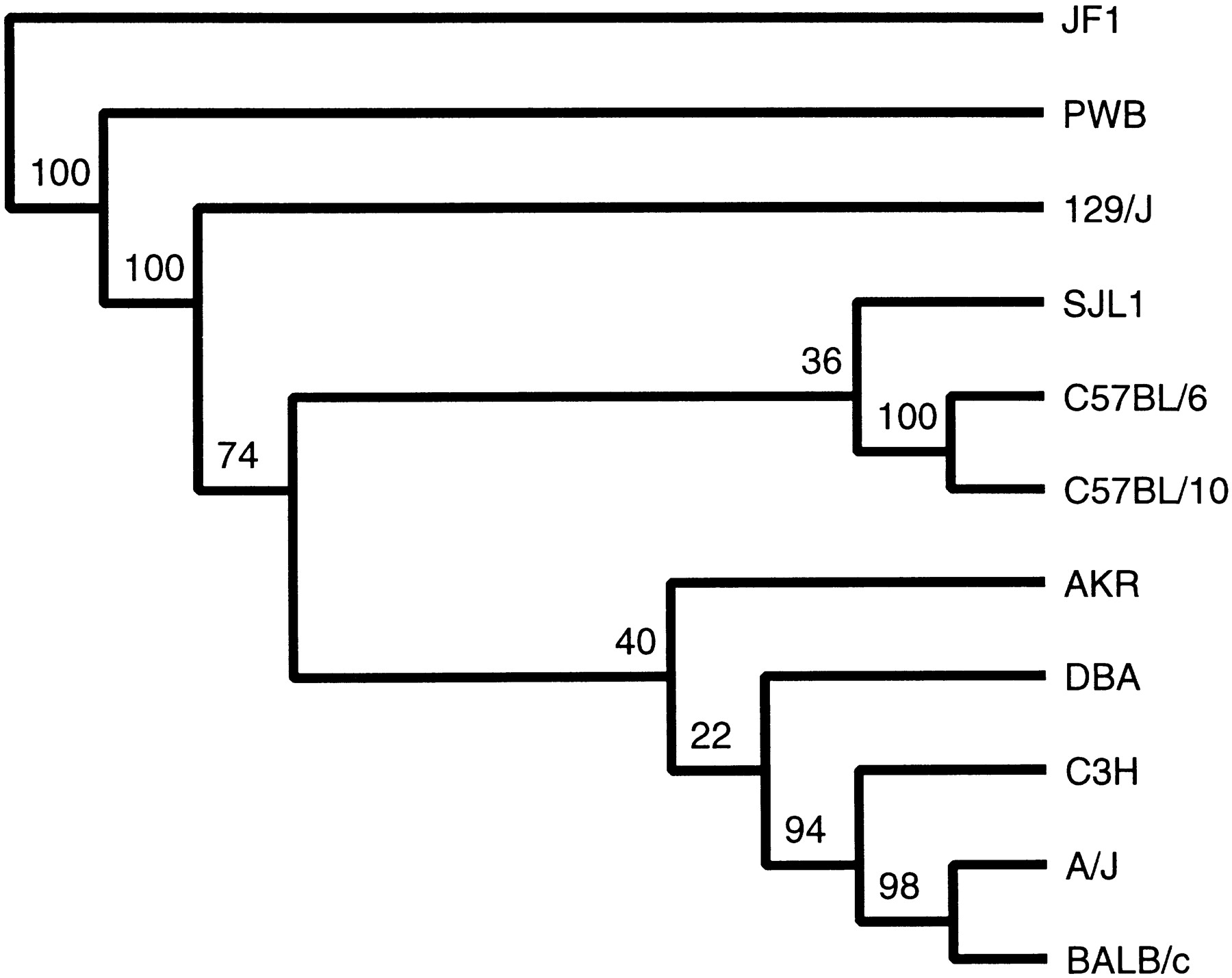
To do the parsimony analysis with PHYLIP 3.5c (Felsenstein 1989) which accepts only binary discrete characters, the microsatellite allele size data were recoded as n − 1 binary discrete characters, where n is the number of alleles (ranging from 2 to 9), in such a way that adjacent sizes differ by one step. This gives an order to the mutational changes between alleles but does not presuppose that a particular allele is ancestral. Thus, for example, if a primer pair gives products sized 102, 104, and 108 bp on our panel of strains, the alleles would be coded using two bits: 00, 01, and 11, respectively. This yields a vector (binary string) of length 520 for each strain. Wagner parsimony analysis was done with the MIX program of PHYLIP (Felsenstein 1989). We tested the robustness of the results by running the analysis on 100 different subsamples of the data (jackknife replicates generated with seqboot), and the consensus tree is shown in Figure 1. The Wagner parsimony method does not assume that the ancestral state is known or that mutation in one direction is more probable than the other. It does, however, assume that species and characters both evolve independently, which perhaps cannot be said of multiple characters (bits) derived from a single microsatellite. Nonetheless, the tree derived is largely congruent with expectations from the known history of the strains and with the analysis of Atchley and Fitch (1991) of 144 single locus genotypes. Most of the branches are highly robust as indicated by jackknife resampling, showing that the observed branching order is not the result of a subset of the recoded data. As expected, the non-domesticus strains, PWB (musculus) and JF1 (molossinus), are distant from each other and from the remaining domesticus strains. Among the domesticus strains, C57BL/6 and C57BL/10 (derived from the same founding pair) form a strongly supported group, as do C3H, A/J, and BALB/c. No unique branching order for SJL/J, AKR, and DBA/2 is supported strongly, which may reflect a more complicated history. Strain 129/J is clearly placed as the most deeply diverged of thedomesticus strains represented. In fact these results provide no evidence that 129/J belongs to the M.m. domesticus group at all, as the tree is unrooted. This nominates 129/J as a good partner for any of the other domesticus strains in terms of polymorphism rate.

Figure 1.

Unrooted consensus tree (of 100 jackknife replicates) derived from microsatellite allele size data by parsimony analysis. Numbers at the forks represent the number of times the group to the right of the fork occurred in 100 jackknife (sampling without replacement) samplings of the data. Branch lengths do not represent distances.

Open in new tab Download PowerPointLink to figure

RH Data

In Table 3, RH linkage, lod score, and distance estimates are presented for each marker relative to the nearest markers in the public RH data, along with the positions of the markers on the genetic map. The high resolution of RH mapping is a consequence of the high break frequency and also means that linkage can be clearly demonstrated only over short distances. Although lod scores are calculated for RH mapping in a way similar to that used for genetic mapping, the data obtained for chromosomes 17 and 13 suggests that high lod scores for linkage are also obtained between markers on different chromosomes. Based on this information, a practical lower linkage lod score limit for placement of unknown markers would be ≥10. A framework having each marker linked to the next with a lod score of 10 would thus be desirable and would require a total of ≥1000 mapped markers. Here we contribute 128 additional markers to this emerging framework and subdivide many of the larger intervals in the McCarthy et al. (1997) data. If independent chromosome assignment is available, the current framework can be used readily to assign markers to the intervals already defined, which correspond to <1 cM for chromosomes 17 and 13 and ∼10 cM for the rest of the genome.

Table 3.

Summary of RH Results

Locus	Pos.	Prev. locus	Pos.	lod	cR	Next locus	Pos.	lod	cR
D1Mit211	15	D1Mit316	8	1.5	108.2	D1Mit171	20.2	3.3	75.7
D1Mit234	26	D1Mit232	21	6.3	51.4	D1Mit236	26	11.7	25.1
D1Mit303	35	D1Mit236	26	2.7	86.0	D1Mit19	37	3.6	73.8
D1Mit332	43	D1Mit46	43	5.8	53.8	D1Mit216	50	5.8	56.0
D1Mit216	50	D1Mit332	43	5.9	56.0	D1Mit10	57	2.7	78.3
D1Mit136	60	D1Mit10	57	3.9	64.6	D1Mit87	62	5.2	57.1
D1Mit446	70	D1Mit286	67	10.0	30.6	D1Mit102	73	7.5	38.9
D1Mit424	82	D1Mit102	73	5.6	50.3	D1Mit33	82	10.6	28.1
D1Mit206	96	D1Mit36	92	6.4	50.3	D1Mit291	102	6.5	48.3
D2Mit117	5	D2Mit312	2	3.5	71.7	D2Mit149	7	5.0	60.1
D2Mit417	22	D2Mit149	7	2.3	90.9	D2Mit365	22	15.0	19.9
D2Mit365	22	D2Mit417	21	15.0	19.9	D2Mit372	27	1.7	103.8
D2Mit372	27	D2Mit365	22	1.8	103.8	D2Mit297	29	4.1	66.8
D2Mit380	40	D2Mit182	37	4.0	68.9	D2Mit44	53	3.1	78.1
D2Mit206	60	D2Mit300	53	7.4	42.9	D2Mit274	62	6.0	49.9
D2Mit525	61	D2Mit106	76	17.2	10.0	D2Mit194	81	7.6	39.6
D2Mit493	72	D2Mit285	86	12.3	22.4	D2Mit263	92	10.9	23.9
D2Mit148	105	D2Mit263	92	7.8	36.8	D2Mit346	92	13.7	19.6
D3Mit130	4	D3Mit264	4	10.6	28.6	D3Mit203	11	1.3	117.8
D3Mit307	22	D3Mit224	22	3.8	65.4	D3Mit22	34	0.0	230.3
D3Mit278	25	D3Mit22	34	6.9	48.5	D3Mit212	40	4.3	67.1
D3Mit77	37	D3Mit29	45	1.8	103.0	D3Mit215	55	1.5	105.6
D3Mit258	70	D3Mit42	59	3.6	73.6	D3Mit84	72	12.4	23.4
D3Mit44	79	D3Mit200	77	19.4	8.0	D3Mit59	84	7.2	48.5
D3Mit87	84	D3Mit59	84	14.0	20.2	D3Mit163	88	11.0	30.0
D4Mit211	6	D4Mit149	12	4.6	2.3	D4Mit94	11	2.8	74.4
D4Mit178	36	D4Mit111	22	1.5	84.2	D4Mit245	43	6.5	50.6
D4Mit166	45	D4Mit245	42	5.9	55.3	D4Mit9	45	13.6	22.6
D4Mit203	60	D4Mit12	57	4.6	51.8	D4Mit54	66	7.6	43.2
D4Mit310	71	D4Mit54	66	8.7	38.9	D4Mit225	80	2.4	79.2
D5Mit346	1	—	—	—	—	D5Mit66	17	0.0	237.5
D5Mit388	18	D5Mit66	17	5.4	58.5	D5Mit78	26	4.0	69.7
D5Mit10	54	D5Mit200	36	2.6	86.3	D5Mit157	57	6.6	50.8
D5Mit25	61	D5Mit240	59	7.2	45.4	D5Mit136	65	8.4	37.4
D5Mit138	69	D5Mit95	68	4.2	65.8	D5Mit221	80	1.1	110.9
D5Mit31	80	D5Mit221	80	14.5	15.2	D5Mit292	83	13.2	22.8
D6Mit139	3	D6Mit138	1	11.8	26.3	D6Mit223	19	1.6	102.7
D6Mit188	33	D6Mit123	29	4.8	61.3	D6Mit8	36	2.7	79.4
D6Mit102	41	D6Mit31	39	16.2	14.2	D6Mit105	46	4.2	67.5
D6Mit105	47	D6Mit102	41	4.3	67.5	D6Mit256	60	4.4	59.6
D6Mit52	61	D6Mit24	57	7.0	46.0	D6Mit289	62	17.7	14.6
D6Mit289	62	D6Mit52	61	17.7	14.6	Kap	64	6.5	46.0
D6Mit14	74	D6Mit259	67	10.7	25.5	D6Mit15	74	9.4	32.2
D7Mit227	16	D7Mit246	15	5.1	58.2	D7Mit69	25	3.7	66.9
D7Mit145	27	D7Mit69	25	8.0	39.2	D7Mit232	27	10.3	30.9
D7Mit31	44	D7Mit176	27	3.6	71.3	D7Mit220	52	2.4	90.1
D7Mit238	53	D7Mit220	52	5.0	60.0	D7Mit165	64	3.7	70.5
D7Mit71	65	D7Mit165	64	1.3	108.2	D7Mit166	66	2.4	89.4
D7Mit46	69	D7Mit12	66	6.5	48.1	—	—	—	—
D8Mit4	14	D8Mit223	11	4.9	61.8	D8Mit191	21	9.9	30.5
D8Mit46	28	D8Mit227	24	0.7	125.5	D8Mit261	33	0.5	146.1
D8Mit242	47	D8Mit184	47	23.0	5.2	D8Mit112	53	0.4	163.0
D8Mit184	47	D8Mit183	47	11.0	23.4	D8Mit242	47	23.0	5.2
D8Mit112	53	D8Mit242	47	0.5	163.0	D8Mit12	53	−0.1	274.9
D8Mit121	67	D8Mit13	67	20.4	5.8	D8Mit93	72	5.6	50.3
D9Mit89	8	D9Mit64	7	14.3	11.7	D9Mit90	9	15.9	14.4
D9Mit269	43	D9Mit207	33	0.6	122.8	D9Mit196	48	6.4	48.9
D9Mit12	55	D9Mit136	54	21.3	5.5	D9Mit182	55	12.0	23.4
D9Mit311	65	D9Mit24	56	5.7	57.3	D9Mit52	72	8.8	35.0
D10Mit183	17	D10Mit86	17	9.0	37.8	D10Mit184	26	1.8	113.6
D10Mit86	17	D10Mit16	16	5.3	57.8	D10Mit183	17	9.0	37.8
D10Mit36	29	D10Mit38	27	7.5	47.5	D10Mit20	32	3.6	74.9
D10Mit38	27	D10Mit184	26	10.6	29.8	D10Mit36	29	7.4	47.5
D10Mit31	36	D10Mit20	32	15.2	13.9	D10Mit42	44	1.9	101.6
D10Mit42	44	D10Mit31	36	2.0	101.6	D10Mit132	47	10.0	34.7
D10Mit132	47	D10Mit42	44	10.1	34.7	D10Mit117	48	13.6	20.7
D10Mit134	59	D10Mit95	51	4.3	64.3	D10Mit136	62	8.0	42.5
D10Mit266	62	D10Mit136	62	13.8	19.9	D10Mit14	65	10.3	26.7
D10Mit271	70	D10Mit14	65	8.4	35.5	—	—	—	—
D11Mit2	2	D11Mit1	1	0.5	154.2	D11Mit227	2	2.5	87.7
D11Mit271	21	D11Mit236	20	14.2	18.4	D11Mit242	31	4.6	64.1
D11Mit242	31	D11Mit271	21	4.6	64.1	D11Mit4	37	9.5	33.3
D11Mit36	48	D11Mit117	45	2.1	101.1	D11Mit213	55	1.3	105.6
D11Mit263	55	D11Mit213	55	13.1	21.3	D11Mit99	60	10.3	31.6
D11Mit224	66	D11Mit166	64	6.9	43.1	D11Mit214	74	1.1	128.0
D11Mit214	74	D11Mit224	66	1.2	128.0	D11Mit69	71	1.5	114.3
D12Mit12	6	D12Mit182	2	3.0	76.8	D12Mit11	6.0	8.8	35.8
D12Mit221	16	D12Mit153	15	9.9	25.9	D12Mit54	24	3.4	75.1
D12Mit201	29	D12Mit54	24	7.4	45.3	D12Mit156	34	6.1	54.3
D12Mit4	34	D12Mit156	34	17.1	12.7	D12Mit158	38	10.2	30.9
D12Mit259	45	D12Mit204	41	5.7	47.8	D12Mit97	47	6.8	43.9
D12Mit167	52	D12Mit97	47	4.3	62.5	D12Mit19	58	4.7	61.1
D12Mit263	58	D12Mit19	58	18.0	10.4	D12Nds2	60	22.1	27.6
D13Mit14	10	D13Mit207	9	7.0	45.3	D13Mit64	30	3.0	81.9
D13Mit64	30	D13Mit14	10	3.0	81.9	D13Mit139	32	6.3	47.6
D13Mit67	37	D13Mit66	37	3.8	69.7	D13Mit125	44	4.2	68.7
D13Mit202	47	D13Mit125	44	10.3	31.3	D13Mit53	62	5.2	59.6
D13Mit53	62	D13Mit202	47	5.2	59.6	D13Mit171	71	10.3	29.8
D14Mit109	3	D14Mit132	1	10.0	26.1	D14Mit11	3	18.6	6.4
D14Mit257	17	D14Mit64	22	9.0	34.0	D14Mit82	20	11.1	26.7
D14Mit158	29	D14Mit82	20	2.2	89.7	D14Mit203	29	14.9	15.9
D14Mit160	40	D14Mit217	33	7.9	38.1	D14Mit67	38	18.7	8.9
D14Mit92	45	D14Mit67	38	6.2	55.7	D14Mit196	47	5.4	49.4
D14Mit97	58	D14Mit75	54	10.3	27.8	D14Mit170	63	8.2	35.5
D15Mit252	10	D15Mit179	11	1.8	93.1	D15Mit136	14	3.4	75.7
D15Mit85	15	D15Mit136	14	2.1	96.8	D15Mit183	23	4.6	63.3
D15Mit270	S	D15Mit183	23	7.5	43.9	D15Mit29	43	5.7	56.2
D15Mit105	42	D15Mit188	44	6.6	46.8	D15Mit107	50	5.4	53.3
D15Mit171	54	D15Mit190	52	22.9	3.6	D15Mit39	57	8.7	36.1
D15Mit14	57	D15Mit193	58	5.1	56.9	D15Mit16	62	5.5	59.2
D16Mit146	17	D16Mit145	14	10.3	25.6	D16Mit57	22	5.0	57.6
D16Mit189	55	D16Mit49	53	4.9	60.7	D16Mit158	55	8.1	40.6
D17Mit133	10	D17Mit196	7	1.9	97.3	D17Mit55	13	14.3	14.5
D17Mit50	23	D17Mit176	23	14.3	12.3	D17Mit52	23	12.6	9.1
D17Mit180	29	D17Mit139	30	10.3	29.3	D17Mit6	31	14.9	16.0
D17Mit185	41	D17Mit119	39	6.5	51.9	D17Mit3	42	9.2	38.3
D17Mit72	47	D17Mit39	45	8.7	41.1	D17Mit73	49	11.0	30.6
D17Mit123	57	D17Mit1	57	3.5	77.0	—	—	—	—
D18Mit60	16	D18Mit147	16	2.7	81.4	D18Mit150	25	4.1	74.9
D18Mit55	25	D18Mit150	25	15.2	16.0	D18Mit123	31	7.4	42.3
D18Mit40	37	D18Mit152	37	7.2	41.1	D18Mit142	47	4.5	58.0
D19Mit56	5	D19Mit59	0	5.4	50.4	D19Mit68	18	4.5	62.0
D19Mit111	15	D19Mit79	6	5.1	61.6	D19Mit40	25	6.8	44.3
D19Mit63	24	D19Mit86	20	1.8	95.5	D19Mit88	34	4.9	63.9
D19Mit88	34	D19Mit63	24	5.0	63.9	D19Mit82	29	3.4	73.2
D19Mit10	47	D19Mit53	43	6.7	41.0	D19Mit91	47	0.2	155.1
D19Mit6	55	D19Mit71	54	15.1	16.6	—	—	—	—
DXMit54	2	DXMit124	3	9.1	35.2	DXMit137	7	11.0	25.4
DXMit81	12	DXMit125	6	7.0	38.9	DXMit49	14	9.4	31.1
DXMit192	19	DXMit50	11	6.8	44.9	DXMit140	19	3.5	62.2
DXMit74	22	DXMit140	19	4.2	54.8	DXMit119	28	6.6	36.7
DXMit170	29	DXMit119	28	3.3	57.6	DXMit95	43	23.0	1.9
DXMit172	40	DXMit149	51	2.9	74.9	DXMit67	60	4.9	57.5
DXMit80	50	DXMit67	60	8.6	35.1	DXMit179	62	6.3	48.9

[i] Data were analyzed using RHMAPPER (Stein et al., 1995), along with all publicly available data (http://www.jax.org). For each marker the lod scores for linkage to the next most centromeric (previous) or telomeric (next) markers are reported as well as the RH distance estimates. Also shown are the genetic map positions of the markers taken from the 1998 Chromosome Committee reports (http://www.jax.org), except for D15Mit52 and D15Mit270, whose positions are from http://www-genome.wi.mit.edu.

Open in new tabLink to table

METHODS

Primers

Oligonucleotides were from TIB MOLBIOL (Berlin, Germany). The reverse primer of each pair was 5′ labeled with the fluorescent dye indicated in Table 1. Many of the primers were redesigned (72 loci marked with an asterisk in the first column of Table 1; primer sequences available http://www.mpimg-berlin-dahlem.mpg.de/∼schalkwy/primer.html). The most common change was the deletion of one or more nucleotides from the 3′ end to avoid overlap with the microsatellite sequence and attendant stuttering artifacts.

DNAs

Mouse T31 RH panel DNAs were from Research Genetics (Huntsville, AL). C3H, SJL/J, and 129/J (stock no. 000690) DNAs were from Jackson Laboratories. PWB and C57BL/10 DNAs were a gift from J. Forejt (Czech Academy of Sciences, Prague). JF1 DNA was a gift from M. Hrabé de Angelis (GSF, Munich, Germany). C57BL/6JOlaHsd (hereafter C57BL/6), AKR/OlaHsd, and A/JOlaHsd were from Harlan Winkelmann (Borchen, Germany). BALB/cJ and DBA/2 DNAs were prepared from mice obtained from OLAC (UK).

For the mouse strain panel, PCR assays were done in a MJ tetrad cycler, using 20-sec denaturation, 20-sec annealing at the temperature given in Table 1, and 20-sec extension at 72°C. Samples with different dyes were pooled and products separated on an ABI 377XL DNA sequencer using internal length standards in every lane. Analysis was with Genescan version 3.0 and Genotyper version 2.1 software from ABI.

RH panel assays were performed as in Schalkwyk et al. (1998): Thirty-microliter reactions with 1.5 mm Mg²⁺ and 6.6 pmoles of each primer were amplified with a 55° touchdown PCR program. For the few primers that did not give easily detectable products under these conditions, amplification was repeated with 3.0 mm Mg²⁺. The products were detected on Southern blots of agarose gels probed with ³²P-labeled (CA)₂₀.

For D8Mit7, RH linkage indicates that the locus is actually on chromosome 9. Genetic mapping gives the same result (J. Walter, unpubl.). This fact may have consequences for the placement of other markers on the MIT map because D8Mit7 is identified as a framework marker.

Parts of this work were funded by the Max-Planck–Gesellschaft and European Union grants BMH4-CT96-0050 (to J.W.) and CT94-0079 (to H.L.).

The publication costs of this article were defrayed in part by payment of page charges. This article must therefore be hereby marked “advertisement” in accordance with 18 USC section 1734 solely to indicate this fact.

Notes

[6] Corresponding author.

[7] Present addresses: ³Ingenium Pharmaceuticals AG, D-82152 Martinsried, Germany; ⁵Genome Pharmaceuticals Corporation AG (GPC AG), Martinsried, Germany.

Notes

[8] E-MAIL [email protected]; FAX 49 30 8413 1380.

REFERENCES

↵
W. AmosS.J. SawcerR.W. FeakesD.C. Rubinsztein(1996) Microsatellites show mutational bias and heterozygote instability. Nat. Genet. 13:390–391.
Google Scholar CrossRef PubMed Web of Science
↵
W.R. AtchleyW.M. Fitch(1991) Gene trees and the origins of inbred strains of mice. Science 254:554–558.
Google Scholar CrossRef PubMed Web of Science
↵
F. BonhommeJ.-L. Guénet(1996) The laboratory mouse and its wild relatives. in Genetic variants and strains of the laboratory mouse, eds M.F. LyonS. RastanS.D.M. Brown3rd ed. , chapter 16, pp. 1537–1576. Oxford University Press, Oxford, UK..
Google Scholar
↵
M. BreenL. DeakinB. MacDonaldS. MillerR. SibsonE. TartellinP. AvnerF. BourgadeJ.-L. GuénetX. Montagutelli(1994) Towards high resolution maps of the mouse and human genomes—A facility for ordering markers to 0.1 cM resolution. Hum. Mol. Genet. 3:621–627.
Google Scholar CrossRef PubMed Web of Science
↵
P. DeloukasG.D. SchulerG. GyapayE.M. BeasleyC. SoderlundP. Rodriguez-ToméL. HuiT.C. MatiseK.B. McKusickJ.S. Beckmann(1998) A physical map of 30,000 human genes. Science 282:744–746.
Google Scholar CrossRef PubMed Web of Science
↵
W.F. DietrichJ. MillerR. SteenM.A. MerchantD. Damron-BolesZ. HusainR. DredgeM.J. DalyK.A. IngallsT.J. O’Conner(1996) A comprehensive genetic map of the mouse genome. Nature 380:149–152.
Google Scholar CrossRef PubMed
↵
R.W. ElliottK.F. ManlyC. Hohman(1999) A radiation hybrid map of mouse chromosome 13. Genomics 57:365–370.
Google Scholar CrossRef PubMed Web of Science
↵
J. Felsenstein(1989) PHYLIP—Phylogeny inference package (v. 3.2). Cladistics 5:164–166.
Google Scholar
↵
M.F.W. Festing(1996) Origins and characteristics of inbred strains of mice. in Genetic variants and strains of the laboratory mouse, eds M.F. LyonS. RastanS.D.M. Brown3rd ed. , chapter 15, pp. 1537–1576. Oxford University Press, Oxford, UK..
Google Scholar
↵
J. ForejtV. VincekJ. KleinH. LehrachM. Loudová-Micková(1991) Genetic mapping of the t-complex region on mouse chromosome 17 including the Hybrid sterility-1 gene. Mamm. Genome 1:84–91.
Google Scholar CrossRef PubMed
↵
T. KoideK. MoriwakiK. UchidaA. MitaT. SagaiH. YonekawaH. KatohN. MiyashitaK. TsuchiyaT.J. NielsenT. Shiroish(1998) New inbred strain JF1 established from Japanese fancy mouse carrying the classic piebald allele. Mamm. Genome 9:15–19.
Google Scholar CrossRef PubMed Web of Science
↵
A. MatinG.B. CollinY. AsadaD. VarnumD. MartoneJ. Nadeau(1998) Simple sequence length polymorphisms that distinguish MOLF/Ei and 129/Sv inbred strains of laboratory mice. Mamm. Genome 9:668–670.
Google Scholar CrossRef PubMed
↵
L.C. McCarthyJ. TerrettM.E. DavisC.J. KnightsA.L. SmithR. CritcherK. SchmittJ. HudsonN.K. SpurrP.N. Goodfellow(1997) A first-generation whole genome-radiation hybrid map spanning the mouse genome. Genome Res. 7:1153–1161.
Google Scholar CrossRef Abstract/Full Text PubMed Web of Science
↵
C.R. PrimmerN. SainoA.P. MøllerH. Ellegren(1998) Unraveling the processes of microsatellite evolution through analysis of germ line mutations in barn swallows Hirundo rustica. Mol. Biol. Evol. 15:1047–1054.
Google Scholar Web of Science
↵
L.C. SchalkwykM. WeiherM. KirbyB. CusackH. HimmelbauerH. Lehrach(1998) Refined radiation hybrid map of mouse chromosome 17. Mamm. Genome 9:807–811.
Google Scholar CrossRef PubMed Web of Science
↵
L.M. Silver(1995) Mouse genetics: Concepts and applications. (Oxford University Press, Oxford, UK).
Google Scholar
↵
Stein, L., L. Kruglyak, D. Slonim, and E. Lander. 1995. “RHMAPPER,” unpublished software, Whitehead Institute/MIT Center for Genome Research. Available at, and, , directory/pub/software/rhmapper. http://www.genome.wi.mit.edu/ftp/pub/software/rhmapper/, ftp.genome.wi.mit.edu.
Google Scholar
↵
J. WeberC. Wong(1993) Mutation of human short tandem repeats. Hum. Mol. Genet. 2:1123–1128.
Google Scholar CrossRef PubMed Web of Science

RESOURCE

Panel of Microsatellite Markers for Whole-Genome Scans and Radiation Hybrid Mapping and a Mouse Family Tree

Current Issue:

Abstract

RESULTS AND DISCUSSION

Mouse Strain Panel Data

Microsatellite Tree

RH Data

METHODS

Primers

DNAs

Notes

Notes

REFERENCES

Article contents

Announcement(s)

RESOURCE

Panel of Microsatellite Markers for Whole-Genome Scans and Radiation Hybrid Mapping and a Mouse Family Tree

Cite this article

Share

Current Issue:

Abstract

RESULTS AND DISCUSSION

Mouse Strain Panel Data

Microsatellite Tree

RH Data

METHODS

Primers

DNAs

Notes

Notes

REFERENCES

Article contents

Announcement(s)