
Abstract
Taxonomic sequence classification is a computational problem central to the study of metagenomics and evolution. Advances in compressed indexing with the r-index enable full-text pattern matching against large sequence collections. But the data structures that link pattern sequences to their clades of origin still do not scale well to large collections. Previous work proposed the document array profiles, which use words of space, where r is the number of maximal equal-letter runs in the Burrows–Wheeler transform, and d is the number of distinct genomes. The linear dependence on d is limiting, because real taxonomies can easily contain 10,000s of leaves or more. We propose a method called cliff compression that reduces this size by a large factor, >250× when indexing the SILVA 16S rRNA gene database. This method uses words of space in expectation under a random model we propose here. We implemented these ideas in an open-source tool called Cliffy that performs efficient taxonomic classification of sequencing reads with respect to a compressed taxonomic index. When applied to simulated 16S rRNA reads, Cliffy's read-level accuracy is higher than Kraken2's by 11%–18%. Clade abundances are also more accurately predicted by Cliffy compared with Kraken2 and Bracken. Overall, Cliffy is a fast and space-economical extension to compressed full-text indexes, enabling them to perform fast and accurate taxonomic classification queries. Cliffy's accuracy underscores the advantages of full-text indexes, which offer a more precise solution compared with k-mer indexes designed for a specific k value.
Compressed indexes are increasingly used for read alignment (Garrison et al. 2018; Armstrong et al. 2020; Sirén et al. 2021) and classification (Ahmed et al. 2021, 2023b) with respect to pangenomes and other collections. These methods exploit the repetitiveness inherent in the Burrows–Wheeler transform (BWT) of a sequence collection by compressing the BWT into its maximal equal-letter runs (Mäkinen and Navarro 2005). Such approaches can straightforwardly determine if a query string is present or absent in the index (Mäkinen and Navarro 2005), but a harder task is to find where the query string occurs. For this, Gagie et al. (2018) proposed a subsampling strategy for the suffix array (SA) along with efficient algorithms for “locate” queries, returning all offsets where the substring occurred. This subsampled SA fits in a space budget of words, where r is the number of BWT runs. Compressed indexes are relevant for taxonomic classification because they enable finding and locating substrings while also compressing away repetitive sequence content. In practice, solving the taxonomic classification problem does not require the full resolution of a locate query. Instead, indexes for taxonomic classification typically support broader queries that either (1) list which in genomes the query string occurs (“document listing”) or (2) find from which portion of the taxonomic tree the substring likely originated (“taxonomic classification”).
We previously introduced a data structure for document listing called document array profiles (Ahmed et al. 2023a). This data structure requires space, where d is the number of genomes (also called “documents”), and enables document listing in time proportional to the number of documents containing the query substring (ndoc). This was the first data structure to enable document listing queries in space proportional to r rather than n. However, the linear dependence on d makes that structure too large for typical taxonomic classification scenarios in which d can be 10,000 or more. For example, the SILVA NR99 SSU reference database (510,508 sequences, 1.2 GB) spans 9118 distinct genera, which would require a document array profile structure >2 TB.
Here, we develop new methods that drastically reduce the space usage. In so doing, we sacrifice the ability to perform full document listing, but we retain the ability to perform accurate taxonomic classification. Detecting and measuring alleles of the 16S rRNA gene allows for the study of bacterial communities, a common task since its introduction in the 1970s (Woese et al. 1975). The gene contains both conserved and hypervariable regions, allowing for primer design (in conserved portions) (Tringe and Hugenholtz 2008; D'Amore et al. 2016) and measurement of evolutionary distance (in variable portions) (Sun et al. 2009; Kim et al. 2014). Projects like the Human Microbiome Project (The Human Microbiome Project Consortium 2012), Earth Microbiome Project (Thompson et al. 2017), and MetaSUB (The MetaSUB Consortium 2016) have used 16S sequencing to characterize the microbes present in the gut, skin, soil, urban environments, and water. In clinical settings, the 16S rRNA gene has been used, for example, to study spatial patterns of microbial infection in lungs of cystic fibrosis patients (Willner et al. 2012), as well as microbial communities in the saliva of Behçet's syndrome patients (Coit et al. 2016).
Existing software tools for 16S rRNA classification use databases such as Greengenes (DeSantis et al. 2006), RDP (Maidak et al. 1997), and SILVA (Quast et al. 2012) as the reference collection. In 2018, Almeida et al. (2018) performed a benchmarking study that showed that QIIME2 (Bolyen et al. 2019) was more accurate than other tools for quantifying reads at the genus and family levels but was computationally very expensive, with time and memory usage 2× and 30× higher, respectively, than other tools. More recently, Lu and Salzberg (2020) extended the popular shotgun metagenomic classifier Kraken2 (Wood et al. 2019) to support 16S rRNA databases, showing that their method was up to 300× faster than QIIME2 while achieving higher accuracy and being the only tool to provide per-read classifications.
Recent innovations in pangenomic indexing also address the scalability and efficiency challenges inherent in classification to large reference collections. Recent methods like Movi (Zakeri et al. 2024), Moni-align (Varki et al. 2025), sampled tag arrays (Depuydt et al. 2025), and chain statistics (Brown et al. 2025) have advanced pangenomic indexing by improving efficiency and accuracy. Movi uses the move structure for cache-efficient backward searches, whereas Moni-align is a full-featured aligner based on the r-index optimized for mapping accuracy. Depuydt et al. (2025) combine the move-structure with a sampled tag array to identify supermaximal exact matches (SMEMs) to use for classification. Chain statistics improve classification resolution by modeling dependencies between hits but require additional storage. In this work, we introduce a method that allows for correct answers to LCA queries over repetitive collections such as 16S databases, which is a functionality not supported by any of those tools.
Our methods are implemented in a new tool called Cliffy that performs per-read 16S rRNA gene classifications using a compressed full-text index. Cliffy uses a novel compression scheme to reduce the size of the document array profiles (Ahmed et al. 2023a) by two orders of magnitude to make it practical for 16S rRNA classification. In addition, Cliffy incorporates strategies such as minimizer digestion and a backward search lookup table to speed up its queries. Using a similar approach to the benchmarking study by Almeida et al. (2018), we generate realistic read data sets from different biomes and show that Cliffy consistently outperforms Kraken2 in terms of per-read accuracy as well as genus abundance profiling. Given Cliffy's accuracy and its capability to find matches of any length, along with the anticipated growth of reference databases, we propose that Cliffy offers a more accurate and scalable alternative to k-mer-based indexes designed for a single value of k.
Methods
Preliminaries
We define a string T[1..n] with length n as a concatenation of characters T[1] · · · T[n] drawn from alphabet Σ of size σ. The empty string, denoted ε, is the only string with length zero. We assume T ends with $ , a special symbol lexicographically smaller than all the symbols in Σ.
Given two integers 1 ≤ i ≤ j ≤ n, we denote T[i..j] = T[i] · · · T[j] as the substring of T spanning positions i to j. Otherwise, if i > j, we define T[i..j] = ε. We refer to T[i..n] as the ith suffix of T and to T[1..i] as the ith prefix of T. Given two strings T[1..n] and S[1..m], lcp(S, T) denotes the length of the longest common prefix (LCP) of T and S.
SA, inverse SA, and longest common prefix array
Given a string T, the suffix array (Manber and Myers 1993) SAT[1..n] is the permutation of {1, …, n} that lexicographically sorts the suffixes of T. The inverse suffix array ISAT[1..n] is the inverse permutation of SAT[1..n], that is, for all i = 1, …, n ISAT[SAT[i]] = i. The longest common prefix array LCPT[1..n] stores the length of the LCP between lexicographically consecutive suffixes of T; formally, LCP[1] = 0, and for all i = 2, …, n, LCP[i] = lcp(T[SAT[i − 1]..n], T[SAS[i]..n]).
Burrows–Wheeler transform
Given a string T, the Burrows–Wheeler transform (Burrows and Wheeler 1994) BWTT[1..n] is a reversible permutation of T defined as the last column of the matrix of the lexicographically sorted rotations of T. When T is terminated by $, we can define for all i = 1, …, n, BWTT[i] = T[SAT[i] − 1], where T[0] = T[n]. LF-mapping is the permutation of {1, …, n} that maps every character in the BWTT to its predecessor in text order; formally, LF[i] = ISAT[SAT[i] − 1] for i, where SAT ≠ 1 and LF[i] = ISAT[n] when SAT = 1. We define r as the number of maximal equal-letter runs of BWTT. When clear from the context, we refer to SAT, ISAT, LCPT, and BWTT as SA, ISA, LCP, and BWT, respectively.
r-index
The r-index (Gagie et al. 2020) is a full-text index based on the run-length encoded BWT and the SA entries sampled at run boundaries. Given a text T[1..n] and a pattern P[1..m], the r-index can locate all occurrences of P in T in time and words of space, where occs is the number of occurrences of P in T.
Document array and document array profiles
We denote a collection of documents (i.e., strings) with , and we denote a concatenation of documents with . The document array (Muthukrishnan 2002) DA[1..n] stores for each position i the document index of . The document array profiles (Ahmed et al. 2023a) are a data structure that enables the r-index to perform document listing queries.
Document listing: Given a collection and a pattern P, return the set of documents where P occurs.
Given an r-index for the concatenated text , the document array profiles supports document listing for a pattern P[1..m] in time and space, where ndoc is the number of documents containing the pattern P.
(From Ahmed et al. [2023a]) Document array profiles: For all positions 1 ≤ LF(i) ≤ n where i is a run head or tail in the BWT of T, the document array profile PDA[i][1..d] stores for each position j = 1, …, d the length of the longest common prefix between and all suffixes of document Tj.
Document listing query using document array profiles
In our previous work (Ahmed et al. 2023a), we demonstrated how to compute a document listing for a pattern P using the document array profiles. The algorithm requires that we store PDA[LF(i)] for all i’s corresponding to a BWT run head or tail, following the “toehold lemma” strategy (Policriti and Prezza 2016); that is, the stored rows are sufficient to recover the document listing for a query pattern P.
Given a query pattern P, we perform a backward search for P and store a pointer to a “sampled” row PDA[i] of the document array profiles, where BWT[i] = P[j], where j is the last character of P that was searched. At each step of the backward search, we either sample a new row or simply increment a counter variable k by one. If the backward search range BWT[s..e] spans a BWT run head or tail, we sample a new row PDA[i], where s ≤ i < e and reset k to zero. Otherwise, if the backward search range is contained within a BWT run, we simply increment k by one.
To generate the document listing, we add k to each value in the “sampled” row PDA[i][1..d] and return all values of j, where PDA[i][j] ≥ |P|. Assuming the LCP values in PDA[i][1..d] are stored in sorted order, we only need to scan the first ndoc + 1 values to generate the document listing. As previously mentioned, the document array profiles supports document listing for a pattern P[1..m] in time and space. More details on the proof for these bounds can be found in the work of Ahmed et al. (2023a).
Taxonomic classification with the pattern lowest common ancestor query
We aim to classify a sequence according to where it likely originated from in the tree of life, represented by a taxonomy. Let a taxonomy R be a rooted multiway tree with d leaves. Given a taxonomy R, we define the collection of documents of the taxonomy, denoted by {R1, …, Rd} as the collection of reference sequences of the taxonomic clades at the leaves of the taxonomy (Fig. 1A). Leaves of the taxonomy R map in a one-to-one fashion with the documents. Internal nodes represent common ancestors and do not have directly associated strings; rather, they are implicitly associated with the union of the documents in the leaves in their subtree. Because a one-to-one mapping exists between leaves and documents, we often refer to these interchangeably.
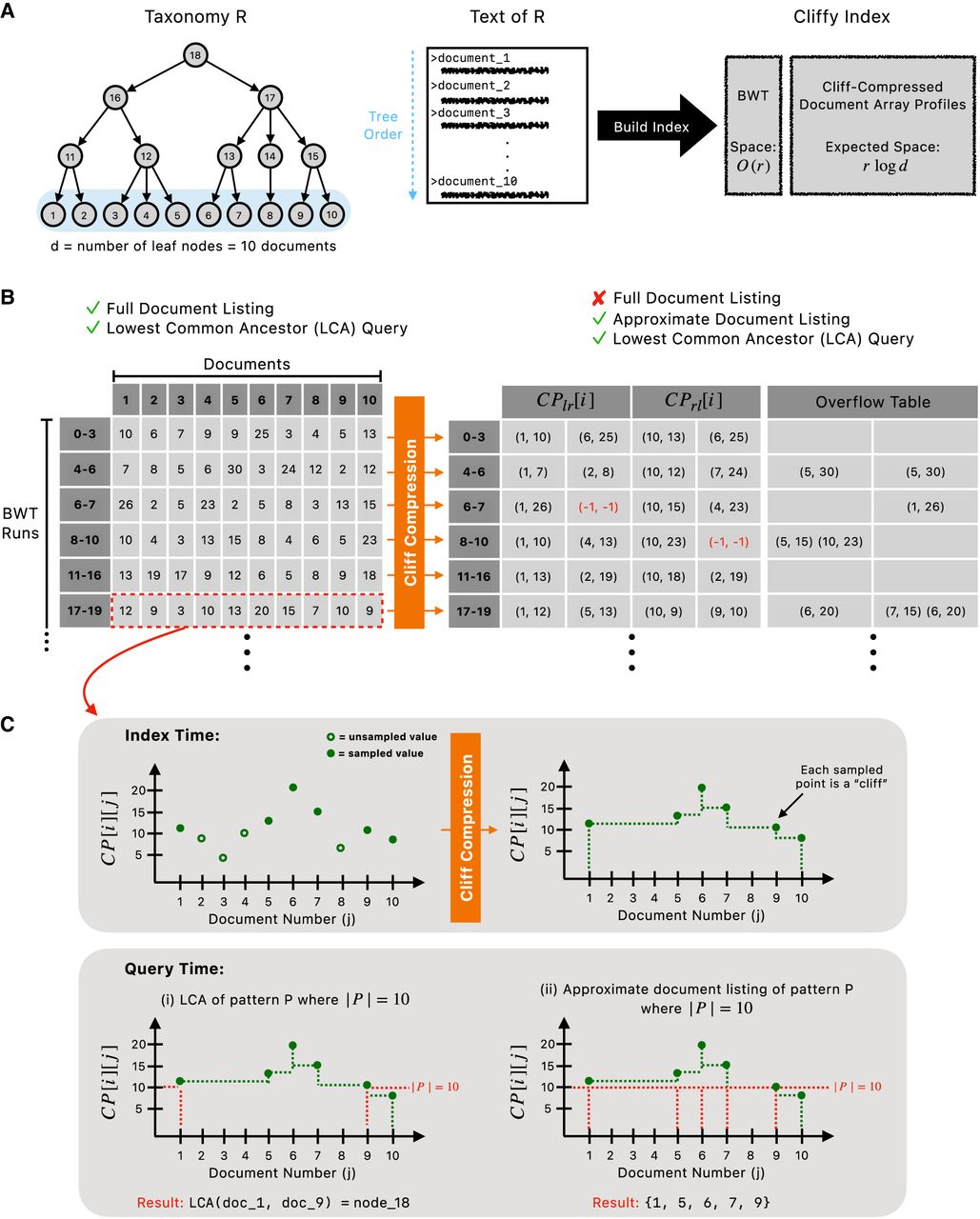
Overview of Cliffy's taxonomy indexing and compression approach. (A) Shows an example taxonomy in which d = 10 and an example tree order that guides the generation of the text of the taxonomy prior to building an index. (B) Visualizes the difference between the document array profiles and the cliff-compressed document array profiles. The cliff-compressed document array profiles consist of a “main table” with a fixed number of columns as well as an “overflow table” that stores any pairs that could not be included in the main table. (C) Using a profile (i.e., row of document array profiles) as an example, it visualizes cliff compression at the index building step, followed by how each profile is used at query time for either the lowest common ancestor query or approximate document listing.
The occurrences of a string P in taxonomy R is the set of leaves F where P occurs as a substring of the associated document.
We summarize where a string P originated using a pattern lowest common ancestor query:
Pattern lowest common ancestor (PLCA): Given a taxonomy R and string P, return the deepest node X such that all of P's occurrences are in leaves of X’s subtree.
To process a set of occurrences of a pattern P in a taxonomy, we define the lowest common ancestor query:
Lowest common ancestor (LCA): Given a taxonomy R and set of nodes F from R, the LCA of F is the deepest node X in R where all nodes in F are present in X’s subtree.
PLCA can be solved by first identifying all occurrences of a pattern P in the leaves and then computing the LCA of those leaves. However, a simpler approach becomes possible if we first consider the leaf nodes to be in a particular order (Gagie et al. 2022):
Tree order: A tree order of the d leaves of taxonomy R is any ordering such that all leaves descended from any internal node are consecutive in the order.
Alternately, we could say that the tree order ensures that descendants of sibling nodes in the tree cannot be interleaved in the order. From here on, we assume that the concatenated text respects tree order for the taxonomy R. We also assume that the document identifications associated with the leaves follow this order; that is, the leftmost (earliest) leaf is document 1, the next is document 2, etc.
(From Gagie et al. [2022]) Assuming tree order, the PLCA query can be answered by computing the LCA of only the leftmost (earliest) and rightmost (latest) leaf nodes containing P in the order.
The proof is by contradiction. We assume a pattern P has occurrences in taxonomy R. Further, we assume the occurrences are sorted by document identifications, such that is an occurrence in the leftmost of the documents that P occurs in, and is an occurrence in the rightmost document that P occurs in. We let denote the LCA of the full set of occurrences and we let LCA() denote the LCA of the leftmost and rightmost occurrences.
We presume . Then it follows that there is a node that occurs either in a document prior to the one matched in occurrence or in a document after the one matched in occurrence . This implies the ordering allows for interleaving of the descendants of sibling nodes, contradicting the assumption of tree ordering.
Given an r-index for a tree-ordered text of a taxonomy extended with the document array profiles PDA, we can compute the PLCA of the pattern P[1..m] in time and words of space.
As summarized in the preliminaries, we previously showed how to compute the document listing for any length substring in time by combining backward search with a scan of a “sampled” row of the document array profiles (Ahmed et al. 2023a). Because we have a tree order, the PLCA for the pattern P can be computed as the LCA of the leftmost and rightmost leaves for which P occurs in their associated document. The LCA of these two leaves is then computed with an auxiliary LCA data structure requiring 2d + o(d) bits of space with query time (Fischer 2010; Navarro 2016). These additional operations are both constant time, ; therefore, total time complexity is .
Shrinking the document array profiles with cliff compression
In the previous section, we proved that we can compute the PLCA for a given pattern using the document array profiles; however, it requires space. We note that in practical settings, d can reach tens of thousands of species (documents). We propose a strategy that we refer to as cliff compression, which has an average space usage of while still allowing for the exact computation of PLCAs. The insight is that to determine the leftmost document containing an ℓ-length match, it is sufficient to identify the smallest j such that PDA[i][j] ≥ ℓ, where i represents the current BWT offset. Similarly, when we ask which is the rightmost document containing an ℓ-length match, it is sufficient to know the largest j such that PDA[i][j] ≥ ℓ. As a result, we only need to store the maxima-so-far, that is, and for all j when they first occur. Although we must store these for both the left-to-right and right-to-left maxima-so-far, the number of instances m where the maxima-so-far changes and we need to store an additional value is small in practice (m ≪ d), making them significantly smaller to store compared with the full document array profile row PDA[i][1..d].
For added intuition, we visualize the profile PDA[i][1..d] (Fig. 1C) with the maxima-so-far step functions drawn as dotted lines. The leftmost and rightmost documents containing a pattern P correspond to the j values where a height-|P| horizontal line crosses the maxima-so-far function. The LCA of the documents at the crossings is the PLCA. Longer matches correspond to higher horizontal lines, which tend to cross a narrower portion of the maxima-so-far function and so lead to deeper PLCAs.
Cliff compression: Given the full document array profiles PDA, we cliff-compress each row by first scanning PDA[i][1..d] from left to right and storing all (j, PDA[i][j]) pairs where j = 1 or . We store these in an array denoted as CPℓr[i], in ascending order by j. We also scan PDA[i][1..d] from right to left and store all (j, PDA[i][j]) pairs, where j = d or . We collect these in an array called CPrℓ[i], in descending order by j. CPℓr and CPrℓ together constitute the cliff-compressed document array profiles.
We can compute PLCAs using only the cliff-compressed document array profiles.
Given the r-index built over the tree-ordered text of a taxonomy , extended with the cliff-compressed document array profiles CPℓr and CPrℓ, we can compute the PLCA for a pattern P in time in words of space.
We adapt the query algorithm given in the preliminaries to work with cliff-compressed document array profiles. Instead of storing PDA[LF[i]] at each head or tail, we store the pair (CPℓr[LF[i]], CPrℓ[LF[i]]). The space usage remains in the worst case. During the backward search, when the range includes a run head or tail, we retrieve (CPℓr[LF[i]], CPrℓ[LF[i]]) for i corresponding to the (contained) head or tail. When the range falls entirely within a run, we obtain our new sample by incrementing each PDA[i][·] value (i.e., LCP) stored in the CPrℓ[i] and CPℓr[i] lists from the previous step by one.
After the backward search, we find the leftmost and rightmost documents containing P. To find the leftmost, we scan the pairs of (j, PDA[i][j]) ∈ CPℓr[i], retrieving the first value j where PDA[i][j] ≥ |P|. By definition of CPℓr, this is the leftmost document containing P. Next, we scan the pairs (j, PDA[i][j]) ∈ CPrℓ[i] and retrieve the first value j such that PDA[i][j] ≥ |P| (recalling that elements of CPrℓ[i] are in descending order by j). By definition of CPrℓ, this is the rightmost document containing P. These scans each require time.
Finally, we query the LCA data structure with leftmost and rightmost documents in time (Fischer 2010; Navarro 2016) to complete the PLCA query. Thus, we can compute the PLCA for a pattern P using the cliff-compressed version of PDA in time.
Random model for cliff-compression ratio
Cliff compression does not improve worst-case space usage compared with the original document array profiles: Both require words of space, with the worst case for cliff compression of CPℓr[i] (resp. CPrℓ[i]) being the case in which the LCP values in PDA[i] are strictly increasing (resp. decreasing). However, we now show that the average-case space complexity when applying cliff compression to the document array profiles is significantly smaller. To accomplish this, we begin by proposing a random model that leads to the average compression ratio of cliff compression, and then, we describe the links between the random model and the cliff-compression scenario.
We model the values in a row i of the document array profiles (PDA[i]) as a random permutation of the d integers 0, 1, …, d − 1. We then consider the “minimum-so-far” computed over the permutation by computing the minimum over all nonempty prefixes of the permutation. We model the number of values we must store in the CPℓr[i] or CPrℓ[i] list as the number of times that the minimum-so-far sequence decreases, plus one. Adding one accounts for the fact that we must always store at least one pair in the array. Note that once the minimum-so-far reaches zero it cannot decrease further.
In practice, the document array profiles deviate from this model. Most importantly, (1) the documents in the taxonomy are related to each other, violating any assumptions of uniform probability of different LCP values, and (2) the values in PDA[i] are not all distinct as in the simple model. Nonetheless, we found that the model was effective at predicting the number of pairs in the cliff-compressed document array profiles (Table 1).
Cliffy index sizes and compression ratios on the SILVA SSU NR99 data set
| Digestion | Document array profiles (Ahmed et al. 2023a) | Cliffy | Reduction ratio | Mean no. of pairs | Variance no. of pairs |
|---|---|---|---|---|---|
| No digestion | 2265 | 9.014 | 251× | 7.095 | 4.633 |
| DNA minimizer | 1955 | 7.858 | 249× | 7.211 | 4.732 |
| Minimizer | 1172 | 4.266 | 275× | 5.137 | 2.664 |
[i] Cliffy index sizes and compression ratios on the SILVA SSU NR99 (510,508 rRNA sequences, d = 9118 genera). Each digestion method shows original size, Cliffy-compressed size, reduction ratio, and pair statistics (mean and variance). The expected mean number of pairs based on harmonic series (H9118 + 1 = 10.695) is discussed in Methods. All sizes are in gigabytes.
Given a random permutation of the n integers 0, 1, …, n − 1, we define the random variable Sn as the number of minima-so-far decreases before reaching zero. The base case is S0 = 0; that is, if the leftmost value in the permutation is zero, then the minimum-so-far is uniformly zero with no decreases. Another easy case is S1 = 1; that is, if the leftmost value is one, then exactly one decrease (to zero) will occur. For S2, we must consider two cases: We reach one before reaching zero, or we reach zero before reaching one. In the first case, S2 = S1 + 1 = 2. In the second, S2 = S0 + 1 = 1. The cases are equally likely because the permutation is random. Therefore, we have . In general, we have
Given the r-index built over the tree-ordered text of a taxonomy , extended with cliff-compressed document array profiles in which the LCPs follow the distribution of random permutations described in the above model, we can compute the PLCA for pattern P in time and words of space.
In Theorem 8, we showed that we can compute the PLCA for a pattern P using the cliff-compressed document array profiles in time in space. Assuming the LCP values in each row of the original document array profiles follow the distribution of random permutations, we prove there is a lower average space bound. In Supplemental Section 2, we show that the expected number of pairs that will be stored in CPℓr[i] and CPrℓ[i] is ; therefore, the total average space for the cliff-compressed document array profiles is .
Approximate document listing
The cliff-compressed document array profiles enable us to perform an additional type of query called approximate document listing. Rather than returning the PLCA of the pattern P, this query returns a subset of the documents in the true document listing for P.
Approximate document listing: Given a sampled cliff-compressed profile, CPℓr[i] and CPrℓ[i], and pattern P, the approximate document listing of P is obtained by scanning all the pairs (j, PDA[i][j]) in both CPℓr[i] and CPrℓ[i]R and returning the set of j, where CPlr,rl[i][j] ≥ |P|.
The motivation for this query is to avoid the potential for vague PLCAs, especially those near the root of the taxonomy. For example, suppose we have a substring M from a read that occurs in n documents, the PLCA of M would be the root of taxonomy even if n − 1 of the occurrences of M were at the left end (earliest) of the tree order and the last occurrence was in the rightmost (latest) document in the tree order. This illustrates a scenario when the PLCA of M gives an unclear classification even though M most likely originated from a document in the left side (earlier) of the tree order.
We note that both the PLCA and approximate document listing queries can be performed by using the same cliff-compressed profile. Even though it fails to be a full document listing, we show in the Results section that the approximate document listing can be a more informative query for classification compared with the PLCA in practice.
Classification methods in Cliffy
Cliffy can perform both read-level classification and abundance profiling. Given a sequencing read, Cliffy begins at the end of the read and performs maximal left-extension using a backward search on the tree-ordered text of the taxonomy. Once the backward search range is empty, Cliffy resets the range to the full BWT at position i, where the previous maximal left-extension ended. Thus, the features for classification used by Cliffy are the exact matches (of varying lengths) between the read and the reference database. Each exact match will have an associated cliff-compressed profile that allows us to compute either the PLCA or the approximate document listing. For example, if we would like to classify at the genus level of the taxonomy and there are d distinct genera, then we initialize a vote array V[1..d] with all zeroes. Next, we iterate through each exact match M and compute the PLCA for M that returns the leftmost ℓ and rightmost r occurrence of M in the taxonomy. We add to all entries between V[l] and V[r], inclusive on both ends, in order to distribute the length of the exact match among all of the leaf nodes in the subtree of the PLCA of M. If we would like to use approximate document listing instead to classify the read, then we consider each exact match M, retrieve the approximate document listing L, and then add to the entries in V corresponding to documents j, where .
Finally, the read is classified by identifying the document j with the maximum value V[j] in V. To perform abundance profiling at the genera level, we classify each read individually and return the proportion of reads classified to each genus.
Running Kraken2/Bracken for classification and profiling
In our experiments, we compared against Kraken2 for read-level classification and the Kraken2+Braken pipeline for abundance profiling. The commands to build the Kraken2/Bracken indexes as well as using them for classification are listed in Supplemental Section 3.
Simulating realistic 16S rRNA data sets
To benchmark Cliffy and Kraken2, we simulated 16S rRNA reads using an approach of Almeida et al. (2018). More specifically, we implemented and used a Python tool called MicrobeMixer that allows us to simulate realistic 16S rRNA reads for different biomes. The commands used can be found in Supplemental Section 4.
Similar to the method previously described (Almeida et al. 2018), we used EBI's MGnify API (Richardson et al. 2023) to query public metagenomic data sets from three different environments (human gut, aquatic, and soil) to identify the top 100 most common genera of bacteria. Next, using the SILVA SSU NR99 database, we take all of the reference sequences for the top 100 genera and extract the sequences in different hypervariable regions (V1–V2, V3–V4, V4, V4–V5) (for exact primers, see Supplemental Section 4) using in silico PCR, for which we allow up to three mismatches in the primer sequence. Next, paired-end sequencing reads 250 bp in length are simulated from these extracted regions using ART (Huang et al. 2012). Finally, MicrobeMixer sampled reads from each of the top 100 genera, mimicking their abundance in the public data, to generate a data set containing 10 million paired-end reads.
Reference digestion with minimizers
Cliffy uses minimizer digestion similar to SPUMONI 2 (Ahmed et al. 2023b) in order to reduce of the size of text prior to indexing. The first type of digestion is the classical case, and we refer to it as “DNA minimizer,” for which we have a small (k) and large (w) window size. The w − k + 1 k-mers in large window are hashed, and the minimizer is the k-mer with the smallest hash value. As Cliffy digests the text, it only concatenates minimizers that are distinct from the preceding one. The second type of digestion treats minimizers themselves as characters opposed to using a “DNA minimizer,” which is a concatenation of k characters. This strategy was previously implemented in assembly-based tools such as mdbg (Ekim et al. 2021) and ntJoin (Coombe et al. 2020). Cliffy uses four for the value of k because with four DNA nucleotides (A, C, G, T) there are 256 possible 4-mers, which can all be represented with 1 byte. Both minimizer approaches allow Cliffy to reduce the size of the text prior to indexing, which in turn reduces the size of the index.
Accelerated querying optimizations in Cliffy
There are two main optimizations in Cliffy that accelerate the query: ftab and minimizer digestion. First, ftab is a lookup table used in a backward search to bypass a prespecified amount of backward search steps inspired by Bowtie 2 (Langmead and Salzberg 2012) and Rowbowt (Mun et al. 2023). In Cliffy, ftab stores the backward search ranges (start and end positions) for all possible 3-mers in the minimizer alphabet. Then at query time, it begins by checking if the 3-mer at the end of the read is present in the text using the ftab; if so, it moves to the fourth character and proceeds with a backward search as normal. Whenever Cliffy resets the backward search range to the full BWT, it will check to see if ftab can be used to accelerate the query.
Second, as previously discussed, Cliffy uses minimizer digestion to reduce both the input text and the reads to shorter sequences. Importantly, this digestion accelerates the query because Cliffy treats each minimizer as its own character; thereby, if k = 4, Cliffy can replace four backward search steps with one.
Results
Experimental setup
We performed the experiments on an Intel Xeon gold 6248R 24-core 3GHz processor with 1500 GB of RAM. We ran on a 64-bit Linux platform. Time was measured using GNU time. Source code and the experimental scripts using Snakemake (Köster and Rahmann 2012) are available on GitHub (see section “Software availability”).
We simulated 12 realistic read data sets from three different environments (“biomes”) and four different hypervariable regions within the 16s rRNA gene. Each read set consisted of 10 million 250 bp Illumina paired-end reads. The exact simulation parameters can found in Supplemental Section 4.
Comparable methods
Other taxonomic classification methods can be broadly categorized as (1) k-mer-based approaches that index the k-mers from the reference, extract k-mers from the read, and use these as keys for finding longer matches (Ounit et al. 2015; Breitwieser et al. 2018; Bolyen et al. 2019; Wood et al. 2019; Şapcı et al. 2024) and (2) full-text approaches that create a full-text index to query with substrings of any length or perform alignments to determine the likely origin of a read (Altschul et al. 1990; Matsen et al. 2010; Kim et al. 2016; Menzel et al. 2016; Ahmed et al. 2023b; Song and Langmead 2024).
A k-mer-based index typically maps k-mers to a summary indicating which taxonomic clades contain the k-mer. Popular tools like Kraken (Wood and Salzberg 2014) and Kraken2 (Wood et al. 2019) store the LCA of the genomes that include the k-mer (or minimizer of the k-mer, in the case of Kraken2). In contrast, full-text-based approaches (Kim et al. 2016; Ahmed et al. 2023b; Song and Langmead 2024), including Cliffy, maintain data structures over the entire reference database to rapidly perform document listing queries on substrings from the sequencing read.
We compare here to Kraken2 because it is the only other method designed for classifying individual 16S rRNA reads rather than abundance profiling. Moreover, although QIIME2 performed well in some prior benchmarking studies (Almeida et al. 2018; Odom et al. 2023), Lu and Salzberg (2020) demonstrated that Kraken2 (Wood et al. 2019) is 300× faster than QIIME2 and achieves higher accuracy; therefore, we focused on comparing to Kraken2. The software versions for the tools tested in the Results are Cliffy (v2.0.0), Kraken2 (v2.1.2), and Bracken (v2.9).
Cliff compression reduces index size substantially
We indexed the SILVA SSU NR99 database (510,508 rRNA gene sequences, 1.2 GB) to classify 16S rRNA reads and observed a substantial compression ratio (249×–275×) for all three index types using different digestion methods (Table 1). For the minimizer index, the average profile storage decreased from d = 9118 values to 5.137 pairs in the cliff-compressed profile, leading to a significant reduction in index size. Based on the simple random model previously described, we expected to store H9118 + 1 = 10.695 pairs after cliff compression. As seen in Table 1, we only needed approximately five to seven pairs on average across the index types. This discrepancy can be explained by the deviations of the real data from the simple model, in which the LCP values are neither all unique nor independent from one another.
Despite this substantial reduction, Kraken2's index remained considerably smaller than Cliffy's index (144 MB vs. 4.266 GB). This is expected because Cliffy is a full-text index and is not limited to a specific k-mer length. In the discussion, we explore additional methods to compress the document array profiles while retaining the ability to perform both LCA and approximate document listing.
Cliffy classifies reads with moderate runtime overhead
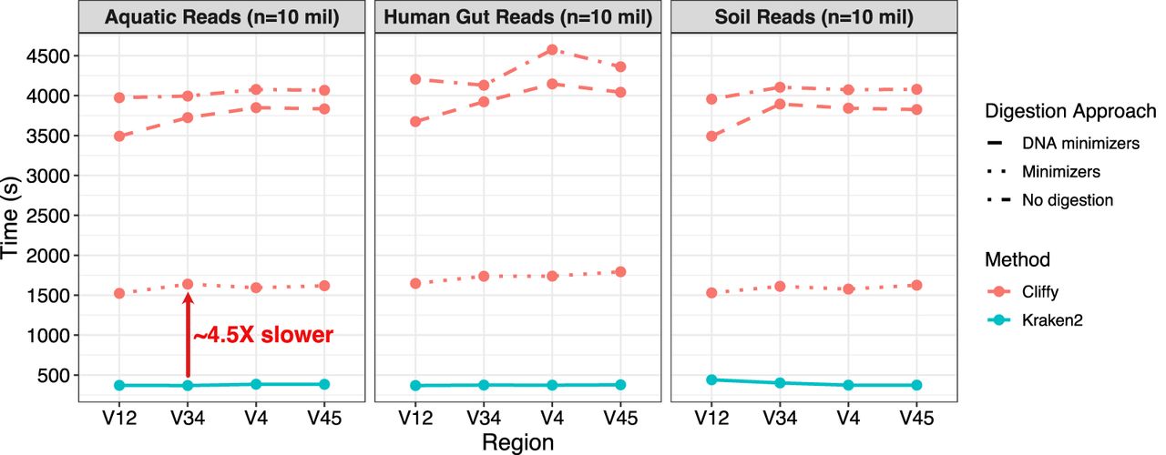
We used both Cliffy and Kraken2 to perform taxonomic read classification over these data sets and measured the running time for both. We observed that although Cliffy was slower than Kraken2 in all its configurations, configuring Cliffy to use its minimizer-based index yielded a running time that was the closest to Kraken2's, being on average 4.5× slower than Kraken2 (Fig. 2). In contrast, Cliffy's other modes are closer to 10×–11× slower. This result is consistent with previous studies (Ekim et al. 2021; Ahmed et al. 2023b) that showed that using minimizers as well as a minimizer-based alphabet can help to speed up read classification. Although the full-text Cliffy index is slower than Kraken 2, we suggest possibilities for improving the efficiency in the discussion.
Classification runtime of Cliffy and Kraken2 on simulated Illumina reads. The figure shows the time required for Cliffy (using approximate document listing) and Kraken2 to classify 10 million simulated Illumina reads (simulated with art_illumina [Huang et al. 2012] using MiSeq v3 error model, 250 bp paired-end). We simulated reads for three different biomes and, for each one, simulated reads from four different hypervariable regions.
Cliffy improves read-level taxonomic assignment accuracy
Having obtained taxonomic classifications for the simulated reads, we next compared Cliffy's classification accuracy to Kraken2's. Although we assess accuracy at all taxonomic levels, we are chiefly concerned with accuracy at the lowest level, which for our 16s RNA taxonomy was the genus level.
Measuring accuracy requires special consideration for the case in which a tool's classification is nonspecific (i.e., not at a leaf of the taxonomic tree) but also correct, in the sense that read's genome of origin is below the node reported by the classifier. In particular, we consider four possibilities: true positives (TPs) are cases in which the read is classified to the correct leaf node of the taxonomy. False positives (FPs) are cases in which the read is classified to a node that is neither the correct leaf node nor an ancestor of the correct leaf node. Vague positives (VPs) are cases in which the read is classified to an ancestor of the correct node. Finally, false negatives (FNs) are cases in which the read is not classified at all by the tool, despite originating from one of the genomes in the taxonomy. Because all simulated reads have their true origin in a node in the taxonomy, true negatives (TNs) are not relevant here. Note that Cliffy reports classifications only at the taxonomic level that is specified by the user; in this case, that was the genus level. Thus, Cliffy does not report any VPs.
To compute accuracy, we divide TP by the total number of reads in the data set. This alone is a useful statistic for Cliffy, but for Kraken2, we additionally report a result for accuracy that includes both TPs and VPs in the numerator. Kraken2 results are shown as a range of values, representing a range of accuracy that depends on whether VPs are considered true or false (gray ribbon in Fig. 3).
Read-level classification accuracy of Cliffy and Kraken2 on the aquatic data set. Shows the read-level classification (n = 10 million Illumina 250 bp paired-end) accuracy for Cliffy and Kraken2 on the Aquatic data set using four different hypervariable regions at different levels of the tree. Each subplot shows Cliffy's performance when using three different types of digestion strategy and two different query approaches: lowest common ancestor and approximate document listing. The gray-shaded region ranges from Kraken2's accuracy when treating all vague positives (VPs) as incorrect compared with treating them all as correct.
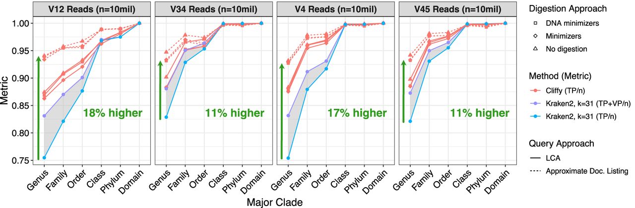
Consistently across the four hypervariable regions, Cliffy had higher accuracy than Kraken2. Cliffy's accuracy percentages ranged from 11 to 18 percentage points higher than Kraken2's at the genus level. This result was consistent across the other two biomes as well (Supplemental Figs. S1, S2). To determine if adjusting Kraken 2's k-mer length would affect the its accuracy, we varied the minimizer length (k) from the default setting of k = 31, namely, the maximum length allowed. We observed that Kraken 2's accuracy decreased when using smaller minimizer lengths (Supplemental Figs. S5–S7). We also observed that Cliffy's more detailed approximate document listing query was consistently more accurate than its LCA query. Finally, when comparing the different digestion approaches, we saw that the default minimizer scheme of k = 4 and w = 11 yielded accuracy results that were nearly identical to those using the full input text with no digestion.
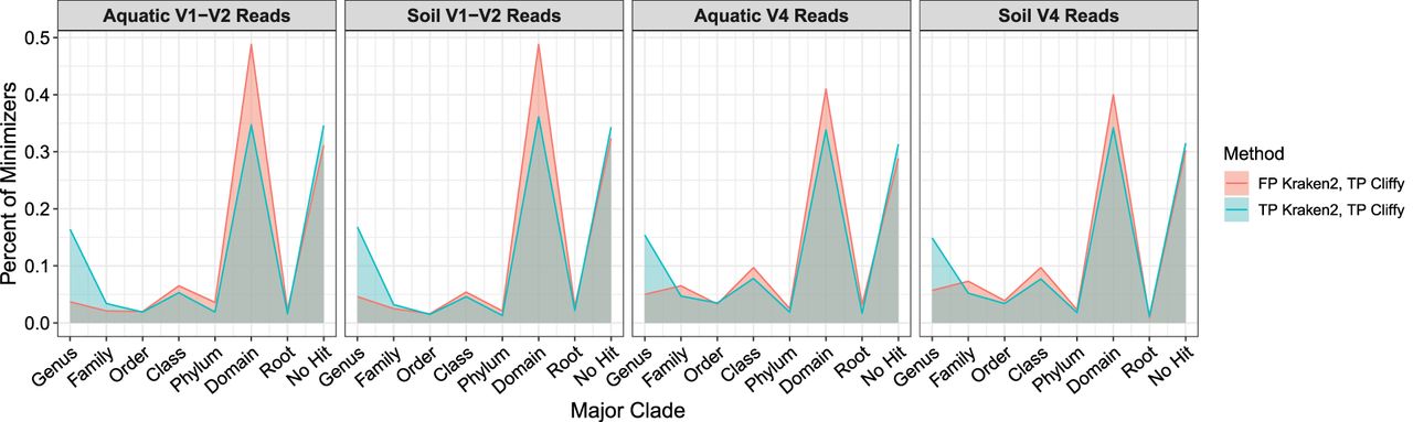
To better understand why Cliffy had a higher accuracy than Kraken2, we focused on the four data sets for which the accuracy gap was the largest. We visualized where in the taxonomy Kraken2 was identifying the LCA nodes for the minimizers it identified from the reads (Fig. 4). When comparing reads that Kraken2 classified correctly versus incorrectly (TP vs. FP), we see that Kraken2 identifies fewer LCA nodes at the genus level and instead finds more at the domain level. Across these four data sets, we see ∼30% of the minimizers are not found in the database (i.e., k is too long), and 30%–50% of the minimizers are at the domain level (i.e., k is too short). These data suggest the minimizer length used by Kraken2 is not always ideal, whereas Cliffy's ability to identify variable length matches allows it to overcome this limitation.
Analysis of minimizer hits to explain accuracy differences between Kraken2 and Cliffy. Focuses on the four data sets with the largest accuracy gap between Kraken2 and Cliffy (using LCA query and not approximate document listing). Looking only at the reads that were false positives for Kraken2 and true positives for Cliffy or reads that were true positives for both tools, we added up the number of minimizers that Kraken2 identified at each level of the taxonomy as well as minimizers that did not hit anything in the database to understand why Kraken2's accuracy was lower than Cliffy despite both tools using the LCA query.
Cliffy accurately estimates genus-level abundances
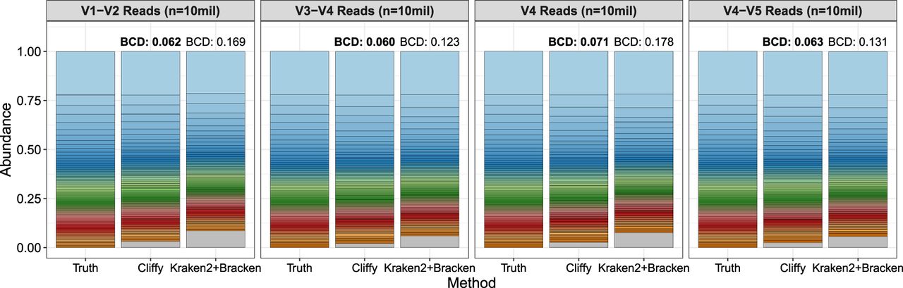
The results discussed so far assessed accuracy at the granularity of individual reads. We further compared these tools at the data set level, comparing their ability to correctly quantify the abundance of each genus. Figure 5 shows the estimated genus-level abundances for the 100 genera simulated in the aquatic data set. For all four regions, Cliffy generated a distribution with the lowest Bray–Curtis distance (BCD) from the true distribution. That trend held as well for the other eight data sets (Supplemental Figs. S3, S4).
Comparison of genera abundance estimates by Cliffy and Kraken2+Bracken on the aquatic data set. Shows the genera abundance results for Cliffy and Kraken2+Bracken for the aquatic data set compared with the truth distribution. Each stacked bar is compared quantitatively with the truth distribution through the Bray–Curtis distance (BCD). The method with the closest distribution to the truth (i.e., lowest BCD) is distinguished with a bold BCD value. The gray section of the Cliffy and Kraken2 bars corresponds to predicted genera that are not truly present in the data set.
Discussion
We introduced Cliffy, which uses a full-text compressed index to perform accurate 16S rRNA gene classifications. We described a novel compression scheme for the document array profiles (Ahmed et al. 2023a), making it far more practical for taxonomic classification. Its use of full-text indexing allows Cliffy to find exact matches of variable length, allowing for greater accuracy compared with Kraken2 (Wood et al. 2019).
The document array profiles (Ahmed et al. 2023a) was the first document listing data structure to have a complexity () that depended only on r and not n, making it particularly practical for repetitive collections like pangenomes. Here we proposed cliff compression, which greatly reduces index size at the expense of enabling only taxonomic classification queries and not full document-listing queries. The compressed index reaches an average size of , which we justified using a random model. Further, we showed that we tend to shrink the index somewhat more than expected in practice. This vast reduction in space makes Cliffy far more practical for taxonomic classification than any past full-text indexing approach.
k-mer-based tools like Kraken2 work by preselecting a particular value for k (e.g., k = 31), but there is no reason to expect any particular value of k is universally appropriate for all sequencing technologies and all portions of the tree of life. Here, we saw evidence both of scenarios in which a fixed value of k was too long (30% minimizers hit nothing in the database), and in which it was too short (30%–50% of minimizers have an LCA at the domain level). In the future, it will be important to continue studying full-text indexes with no preselection of k, as this could be critical to enabling high accuracy over time and over various technologies and clades.
Despite the query optimizations and compression, the main weakness of Cliffy is its lower computational efficiency compared with the k-mer-based Kraken2 method. Currently, Kraken2 is ∼4.5× faster at classifying reads compared with Cliffy when using minimizer digestion. Also, Kraken2's index is ∼30× smaller (4.266 GB vs. 144 MB). Although this work represents a major closing of the index-size gap, we will continue to look for opportunities to close the gap in terms of both speed and index size. To reduce query time, we could consider using faster rank queries that could potentially speed up the backward search step in Cliffy's code for finding pattern matches (Díaz-Domínguez et al. 2023; Ceregini et al. 2024). Further speed improvement could come from using an alternative data structure for the run-length-compressed BWT, such as move-structure (Nishimoto et al. 2022; Zakeri et al. 2024), which allows for a faster backward search (up to 30× faster than current approaches) at the cost of a larger index.
To reduce Cliffy's index size, we can exploit the inherent feature of cliff compression in which the stored profile values (CPℓr,rℓ[i][j]) are strictly increasing; therefore, we could use a delta-encoding scheme to reduce the memory needed to store them. Recent works in k-mer indexes have used exploited the repetitiveness of colors to reduce the size of their indexes (Fan et al. 2024). It is possible a similar approach can be applied to the cliff-compressed document array profiles if groups of document identifications tend to be stored together after applying the compression. Currently, this limitation is what makes it difficult for Cliffy to be applied directly to whole-genome databases such as GTDB (Parks et al. 2020), and initial experiments show that Cliffy's memory footprint grows rapidly when dealing with these large reference sequences (Supplemental Fig. S8; Supplemental Table S1). Future work will focus on improving the construction algorithm to reduce the temporary disk footprint by parallelizing the construction and compressing the rows of the document array profiles on the fly as opposed to delaying it till the end of the algorithm.
Although this study evaluated Cliffy only in the context of 16s RNA analysis, the underlying algorithms and cliff compression are applicable in any taxonomic classification setting, including for whole-genome shotgun metagenomics. As with k-mer indexes or any other compressed index, it is always crucial to evaluate the achieved compression ratio. We observed that 16S rRNA sequences enable an impressive compression ratio of around 18-fold, meaning the n/r ratio achieved by the r-index was about 18. When applying these methods to other databases, the compression ratio could vary, and other compressed indexing methods, such as the one used by Centrifuger (Song and Langmead 2024), might be more appropriate.
Software availability
The Cliffy software and the code for reproducing the experimental results presented in this study are available at GitHub (https://github.com/oma219/cliffy and https://github.com/oma219/cliffy-experiments, respectively), and as Supplemental Code.
Competing interest statement
The authors declare no competing interests.
Acknowledgments
We thank the Advanced Research Computing at Hopkins (ARCH) core facility (https://www.arch.jhu.edu/) for providing computational resources. ARCH is supported by the National Science Foundation, Directorate for Computer and Information Science and Engineering, under grant OAC-1920103. This work was also supported by the National Science Foundation, Directorate for Biological Sciences, under grant DBI-2029552 and by the National Institutes of Health under grants R01HG011392, R35GM139602, and T32GM119998. We also acknowledge the SILVA rRNA database maintainers for providing publicly available reference collections and the open-source software community for their contributions used in this study.
Author contributions: Conceptualization was by O.A. and B.L. Methodology was by O.A. and C.B. Software was by O.A. Investigation was by O.A. Writing of the original draft was by O.A. Reviewing and editing were by O.A., C.B., and B.L. Supervision was by C.B. and B.L. All author approved the final version.
Notes
[2] Supplementary material [Supplemental material is available for this article.]
[3] Article published online before print. Article, supplemental material, and publication date are at https://www.genome.org/cgi/doi/10.1101/gr.279846.124.
References
- ↵Ahmed O, Rossi M, Kovaka S, Schatz MC, Gagie T, Boucher C, Langmead B. 2021. Pan-genomic matching statistics for targeted nanopore sequencing. iScience 24: 102696. 10.1016/j.isci.2021.102696
- ↵Ahmed O, Rossi M, Boucher C, Langmead B. 2023a. Efficient taxa identification using a pangenome index. Genome Res 33: 1069–1077. 10.1101/gr.277642.123
- ↵Ahmed OY, Rossi M, Gagie T, Boucher C, Langmead B. 2023b. SPUMONI 2: improved classification using a pangenome index of minimizer digests. Genome Biol 24: 122. 10.1186/s13059-023-02958-1
- ↵Almeida A, Mitchell AL, Tarkowska A, Finn RD. 2018. Benchmarking taxonomic assignments based on 16S rRNA gene profiling of the microbiota from commonly sampled environments. GigaScience 7: giy054. 10.1093/gigascience/giy054
- ↵Altschul SF, Gish W, Miller W, Myers EW, Lipman DJ. 1990. Basic local alignment search tool. J Mol Biol 215: 403–410. 10.1016/S0022-2836(05)80360-2
- ↵Armstrong J, Hickey G, Diekhans M, Fiddes IT, Novak AM, Deran A, Fang Q, Xie D, Feng S, Stiller J, 2020. Progressive Cactus is a multiple-genome aligner for the thousand-genome era. Nature 587: 246–251. 10.1038/s41586-020-2871-y
- ↵Bolyen E, Rideout JR, Dillon MR, Bokulich NA, Abnet CC, Al-Ghalith GA, Alexander H, Alm EJ, Arumugam M, Asnicar F, 2019. Reproducible, interactive, scalable and extensible microbiome data science using QIIME 2. Nat Biotechnol 37: 852–857. 10.1038/s41587-019-0209-9
- ↵Breitwieser FP, Baker DN, Salzberg SL. 2018. KrakenUniq: confident and fast metagenomics classification using unique k-mer counts. Genome Biol 19: 198. 10.1186/s13059-018-1568-0
- ↵Brown NK, Shivakumar VS, Langmead B. 2025. Improved pangenomic classification accuracy with chain statistics. In Research in computational molecular biology: lecture notes in computer science, Vol. 15647 (ed. Sankararaman S), pp. 190–208. Springer, Cham, Switzerland.
- ↵Burrows M, Wheeler DJ. 1994. A block sorting lossless data compression algorithm: technical report 124, Digital Equipment Corporation, Palo Alto, CA.
- ↵Ceregini M, Kurpicz F, Venturini R. 2024. Faster wavelet tree queries. In 2024 Data Compression Conference (DCC), Snowbird, UT, pp. 223–232. IEEE, Piscataway, NJ.
- ↵Coit P, Mumcu G, Ture-Ozdemir F, Unal AU, Alpar U, Bostanci N, Ergun T, Direskeneli H, Sawalha AH. 2016. Sequencing of 16S rRNA reveals a distinct salivary microbiome signature in Behcet's disease. Clin Immunol 169: 28–35. 10.1016/j.clim.2016.06.002
- ↵Coombe L, Nikolić V, Chu J, Birol I, Warren RL. 2020. ntJoin: fast and lightweight assembly-guided scaffolding using minimizer graphs. Bioinformatics 36: 3885–3887. 10.1093/bioinformatics/btaa253
- ↵D'Amore R, Ijaz UZ, Schirmer M, Kenny JG, Gregory R, Darby AC, Shakya M, Podar M, Quince C, Hall N. 2016. A comprehensive benchmarking study of protocols and sequencing platforms for 16S rRNA community profiling. BMC Genomics 17: 55. 10.1186/s12864-015-2194-9
- ↵Depuydt L, Ahmed OY, Fostier J, Langmead B, Gagie T. 2025. Run-length compressed metagenomic read classification with SMEM-finding and tagging. bioRxiv 10.1101/2025.02.25.640119
- ↵DeSantis TZ, Hugenholtz P, Larsen N, Rojas M, Brodie EL, Keller K, Huber T, Dalevi D, Hu P, Andersen GL. 2006. Greengenes, a chimera-checked 16S rRNA gene database and workbench compatible with ARB. Appl Environ Microbiol 72: 5069–5072. 10.1128/AEM.03006-05
- ↵Díaz-Domínguez D, Dönges S, Puglisi SJ, Salmela L. 2023. Simple runs-bounded FM-index designs are fast. In Proceedings of the 21st International Symposium on Experimental Algorithms (SEA), pp. 7:1–7:16. Schloss-Dagstuhl-Leibniz Zentrum für Informatik, Wadern, Germany.
- ↵Ekim B, Berger B, Chikhi R. 2021. Minimizer-space de Bruijn graphs: whole-genome assembly of long reads in minutes on a personal computer. Cell Syst 12: 958–968.e6. 10.1016/j.cels.2021.08.009
- ↵Fan J, Khan J, Singh NP, Pibiri GE, Patro R. 2024. Fulgor: a fast and compact k-mer index for large-scale matching and color queries. Algorithms Mol Biol 19: 3. 10.1186/s13015-024-00251-9
- ↵Fischer J. 2010. Optimal succinctness for range minimum queries. In Latin American Symposium on Theoretical Informatics, Oaxaca, Mexico, pp. 158–169. Springer, Berlin, Heidelberg.
- ↵Gagie T, Navarro G, Prezza N. 2018. Optimal-time text indexing in BWT-runs bounded space. In Proceedings of the 29-th Annual ACM-SIAM Symposium on Discrete Algorithms (SODA), New Orleans, pp. 1459–1477. Society for Industrial and Applied Mathematics, Philadelphia.
- ↵Gagie T, Navarro G, Prezza N. 2020. Fully functional suffix trees and optimal text searching in BWT-runs bounded space. J ACM 67: 2:1–2:54. 10.1145/3375890
- ↵Gagie T, Kashgouli S, Langmead B. 2022. KATKA: A Kraken-like tool with k given at query time. In International Symposium on String Processing and Information Retrieval (SPIRE), Concepción, Chile, pp. 191–197. Springer, Berlin, Heidelberg.
- ↵Garrison E, Sirén J, Novak AM, Hickey G, Eizenga JM, Dawson ET, Jones W, Garg S, Markello C, Lin MF, 2018. Variation graph toolkit improves read mapping by representing genetic variation in the reference. Nat Biotechnol 36: 875–879. 10.1038/nbt.4227
- ↵Huang W, Li L, Myers JR, Marth GT. 2012. Art: a next-generation sequencing read simulator. Bioinformatics 28: 593–594. 10.1093/bioinformatics/btr708
- ↵The Human Microbiome Project Consortium. 2012. Structure, function and diversity of the healthy human microbiome. Nature 486: 207–214. 10.1038/nature11234
- ↵Kim M, Oh H-S, Park S-C, Chun J. 2014. Towards a taxonomic coherence between average nucleotide identity and 16S rRNA gene sequence similarity for species demarcation of prokaryotes. Int J Syst Evol Microbiol 64: 346–351. 10.1099/ijs.0.059774-0
- ↵Kim D, Song L, Breitwieser FP, Salzberg SL. 2016. Centrifuge: rapid and sensitive classification of metagenomic sequences. Genome Res 26: 1721–1729. 10.1101/gr.210641.116
- ↵Köster J, Rahmann S. 2012. Snakemake—a scalable bioinformatics workflow engine. Bioinformatics 28: 2520–2522. 10.1093/bioinformatics/bts480
- ↵Langmead B, Salzberg SL. 2012. Fast gapped-read alignment with Bowtie 2. Nat Methods 9: 357–359. 10.1038/nmeth.1923
- ↵Lu J, Salzberg SL. 2020. Ultrafast and accurate 16S rRNA microbial community analysis using Kraken 2. Microbiome 8: 124. 10.1186/s40168-020-00900-2
- ↵Maidak BL, Olsen GJ, Larsen N, Overbeek R, McCaughey MJ, Woese CR. 1997. The RDP (Ribosomal Database Project). Nucleic Acids Res 25: 109–110. 10.1093/nar/25.1.109
- ↵Mäkinen V, Navarro G. 2005. Succinct suffix arrays based on run-length encoding. In Proceedings of the 16th Annual Symposium Combinatorial Pattern Matching (CPM), Seoul, South Korea, pp. 45–56. Springer-Verlag, Berlin, Heidelberg.
- ↵Manber U, Myers G. 1993. Suffix arrays: a new method for on-line string searches. SIAM J Comput 22: 935–948. 10.1137/0222058
- ↵Matsen FA, Kodner RB, Armbrust EV. 2010. pplacer: linear time maximum-likelihood and Bayesian phylogenetic placement of sequences onto a fixed reference tree. BMC Bioinformatics 11: 538. 10.1186/1471-2105-11-538
- ↵Menzel P, Ng KL, Krogh A. 2016. Fast and sensitive taxonomic classification for metagenomics with Kaiju. Nat Commun 7: 11257. 10.1038/ncomms11257
- ↵The MetaSUB Consortium. 2016. The metagenomics and metadesign of the subways and urban biomes (MetaSUB) international consortium inaugural meeting report. Microbiome 4: 24. 10.1186/s40168-016-0168-z
- ↵Mun T, Vaddadi NSK, Langmead B. 2023. Pangenomic genotyping with the marker array. Algorithms Mol Biol 18: 2. 10.1186/s13015-023-00225-3
- ↵Muthukrishnan S. 2002. Efficient algorithms for document retrieval problems. In Proceedings of the ACM-SIAM Symposium on Discrete Algorithms (SODA), San Francisco, pp. 657–666. Society for Industrial and Applied Mathematics, Philadelphia.
- ↵Navarro G. 2016. Compact data structures: a practical approach. Cambridge University Press, Cambridge.
- ↵Nishimoto T, Kanda S, Tabei Y. 2022. An optimal-time RLBWT construction in BWT-runs bounded space. In Proceedings of the International Colloquium on Automata, Languages, and Programming (ICALP), Vol. 229, Paris, pp. 99:1–99:20. Schloss-Dagstuhl-Leibniz-Zentrum für Informatik, Wadern, Germany.
- ↵Odom AR, Faits T, Castro-Nallar E, Crandall KA, Johnson WE. 2023. Metagenomic profiling pipelines improve taxonomic classification for 16S amplicon sequencing data. Sci Rep 13: 13957. 10.1038/s41598-023-40799-x
- ↵Ounit R, Wanamaker S, Close TJ, Lonardi S. 2015. CLARK: fast and accurate classification of metagenomic and genomic sequences using discriminative k-mers. BMC Genomics 16: 236. 10.1186/s12864-015-1419-2
- ↵Parks DH, Chuvochina M, Chaumeil P-A, Rinke C, Mussig AJ, Hugenholtz P. 2020. A complete domain-to-species taxonomy for bacteria and archaea. Nat Biotechnol 38: 1079–1086. 10.1038/s41587-020-0501-8
- ↵Policriti A, Prezza N. 2016. Computing LZ77 in run-compressed space. In Proceedings of the Data Compression Conference (DCC), Snowbird, UT, pp. 23–32. IEEE, Piscataway, NJ.
- ↵Quast C, Pruesse E, Yilmaz P, Gerken J, Schweer T, Yarza P, Peplies J, Glöckner FO. 2012. The SILVA ribosomal RNA gene database project: improved data processing and web-based tools. Nucleic Acids Res 41: D590–D596. 10.1093/nar/gks1219
- ↵Richardson L, Allen B, Baldi G, Beracochea M, Bileschi ML, Burdett T, Burgin J, Caballero-Pérez J, Cochrane G, Colwell LJ, 2023. MGnify: the microbiome sequence data analysis resource in 2023. Nucleic Acids Res 51: D753–D759. 10.1093/nar/gkac1080
- ↵Şapcı AOB, Rachtman E, Mirarab S. 2024. CONSULT-II: accurate taxonomic identification and profiling using locality-sensitive hashing. Bioinformatics 40: btae150. 10.1093/bioinformatics/btae150
- ↵Sirén J, Monlong J, Chang X, Novak AM, Eizenga JM, Markello C, Sibbesen JA, Hickey G, Chang P-C, Carroll A, 2021. Pangenomics enables genotyping of known structural variants in 5202 diverse genomes. Science 374: abg8871. 10.1126/science.abg8871
- ↵Song L, Langmead B. 2024. Centrifuger: lossless compression of microbial genomes for efficient and accurate metagenomic sequence classification. Genome Biol 25: 106. 10.1186/s13059-024-03244-4
- ↵Sun Y, Cai Y, Liu L, Yu F, Farrell ML, McKendree W, Farmerie W. 2009. ESPRIT: estimating species richness using large collections of 16S rRNA pyrosequences. Nucleic Acids Res 37: e76. 10.1093/nar/gkp285
- ↵Thompson LR, Sanders JG, McDonald D, Amir A, Ladau J, Locey KJ, Prill RJ, Tripathi A, Gibbons SM, Ackermann G, 2017. A communal catalogue reveals earth's multiscale microbial diversity. Nature 551: 457–463. 10.1038/nature24621
- ↵Tringe SG, Hugenholtz P. 2008. A renaissance for the pioneering 16S rRNA gene. Curr Opin Microbiol 11: 442–446. 10.1016/j.mib.2008.09.011
- ↵Varki R, Rossi M, Ferro E, Oliva M, Garrison E, Langmead B, Boucher C. 2025. Accurate short-read alignment through r-index-based pangenome indexing. Genome Res 35: 1609–1620. 10.1101/gr.279858.124
- ↵Willner D, Haynes MR, Furlan M, Schmieder R, Lim YW, Rainey PB, Rohwer F, Conrad D. 2012. Spatial distribution of microbial communities in the cystic fibrosis lung. ISME J 6: 471–474. 10.1038/ismej.2011.104
- ↵Woese CR, Fox GE, Zablen L, Uchida T, Bonen L, Pechman K, Lewis BJ, Stahl D. 1975. Conservation of primary structure in 16S ribosomal RNA. Nature 254: 83–86. 10.1038/254083a0
- ↵Wood DE, Salzberg SL. 2014. Kraken: ultrafast metagenomic sequence classification using exact alignments. Genome Biol 15: R46. 10.1186/gb-2014-15-3-r46
- ↵Wood DE, Lu J, Langmead B. 2019. Improved metagenomic analysis with Kraken 2. Genome Biol 20: 257. 10.1186/s13059-019-1891-0
- ↵Zakeri M, Brown NK, Ahmed OY, Gagie T, Langmead B. 2024. Movi: a fast and cache-efficient full-text pangenome index. iScience 27: 111464. 10.1016/j.isci.2024.111464