Abstract
Accurate detection of mutations within bacterial species is critical for fundamental studies of microbial evolution, reconstruction of transmission events, and identification of antimicrobial resistance mutations. Although many tools have been developed to identify single-nucleotide variants (SNVs) from whole-genome sequencing, they often suffer from high false-positive rates owing to the complexity of bacterial genomes and the need for different filtering cutoffs across sample types and sequencing depths. As data sets increase in size, the manual filtering required for high accuracy presents a significant obstacle. Here, we present AccuSNV, a novel deep learning–based tool for high-precision and automated bacterial SNV calling. Unlike traditional methods that process one sample at a time, AccuSNV leverages a convolutional neural network (CNN) that integrates alignment information across multiple samples, enhancing precision through learned across-sample patterns. We evaluate AccuSNV against seven popular SNV-calling tools using simulated data from six bacterial species with varied sequencing depths, numbers of isolates, mutations, and divergence levels. To further validate its real-world utility, we test AccuSNV on multiple curated bacterial data sets containing reported SNVs. In both simulated and real-world scenarios, AccuSNV consistently achieves the best performance. Moreover, AccuSNV provides comprehensive user-friendly downstream analysis modules and outputs, including mutation annotation information, phylogenetic inference, dN/dS calculations, and optional manual filtering. Together with the automated deep learning–based calling, these features make AccuSNV broadly accessible to users with different levels of computational expertise.
Single-nucleotide variants (SNVs), single-base substitutions in a genome, represent the most common form of genetic variation. In bacteria, accurate identification of SNVs is a critical step in connecting genetic variation to the phenotype (Lopatkin et al. 2021; Schrader et al. 2021) and for reconstructing bacterial evolution (Barrick et al. 2009). In particular, SNV mutations form the basis of most phylogenetic inference approaches, making their accurate detection essential for epidemiology (Halachev et al. 2014). Even small errors in SNV detection can have outsized effects on downstream analyses. This is especially true for many bacterial species, which accumulate SNV mutations at a rate of only one to 10 SNVs per genome per year (Key et al. 2023). This low rate of mutation accumulation makes evolutionary inference methods sensitive to false positives, thus requiring high-precision SNV calling.
SNV calling across bacterial genomes of the same species remains a challenging task. One major source of SNV-calling errors arises from alignment inaccuracies, which are exacerbated by the high diversity within bacterial species. Unlike the relatively stable and homogeneous human genome, bacteria within the same species can vary up to 5% in nucleotide identity and share only 40% of their gene content. These characteristics increase the possibility of misalignments and false variant calls (Zojer et al. 2017), particularly in low-coverage data sets or when the sample strain diverges from the reference genome (Bush et al. 2020). In addition, cross-contamination during high-throughput sequencing preparation can lead to false-positive and false-negative SNV calls, posing challenges for standard mapping-based SNV filtering methods (Goig et al. 2020). These errors can significantly reduce the precision of bacterial SNV calling.
Several SNV-calling tools have been developed and applied to identify SNVs across bacterial isolates (Koboldt et al. 2009; Li et al. 2009; McKenna et al. 2010; Garrison and Marth 2012; Barrick et al. 2014; Yoshimura et al. 2019). Most of these tools combine probabilistic models (likelihoods or statistics) for each genotype in each sample based on alignment metrics such as base quality, read depth, and strand bias and then apply filters or thresholds to make allele calls in per-sample basis. Some of these tools, such as GATK and FreeBayes, were originally designed for eukaryotic organisms like humans (McKenna et al. 2010) and are not specifically optimized for bacterial genomes, whereas others like breseq and Snippy are tailored for microbial analysis. These methods are widely used owing to their simplicity and informative visualizations that support additional filtering as needed. A second category integrates both mapping and assembly information. For example, BactSNP performs de novo assembly of input reads and aligns the assembled contigs to the reference genome to identify SNVs. Through this approach, BactSNP aims to reduce false positives caused by read misalignment in complex genomic regions. However, the accuracy of this approach depends heavily on the quality of the assembly and the similarity between sample and reference genomes, and it remains computationally intensive for large data sets (Supplemental Table S1).
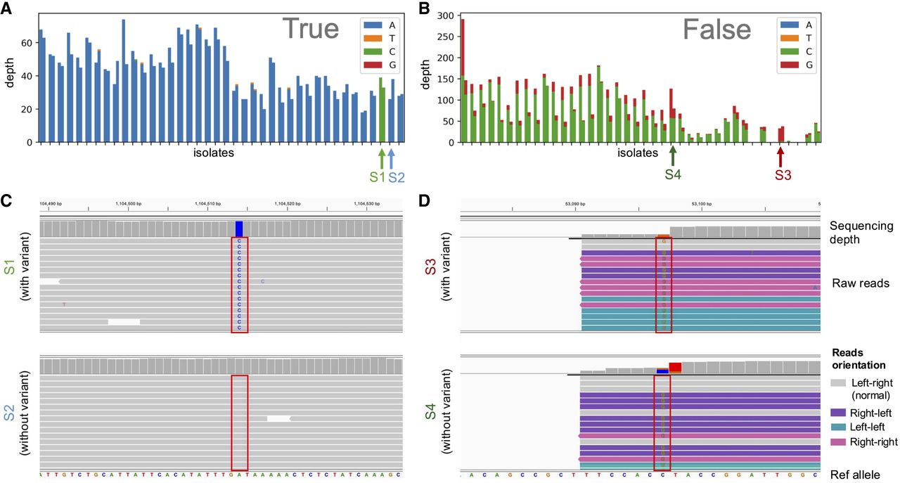
Despite their respective strengths, these existing methods share common limitations. First, most tools typically call variants by considering each isolate individually, which obscures across-sample patterns that can reveal systematic alignment errors at specific genomic positions. False SNVs emerging from alignment errors exhibit distinct alignment patterns across samples (Fig. 1A–D), and failing to consider these patterns while focusing solely on single-sample evidence can lead to false-positive calls. Another common issue is reference bias: When all samples share a nucleotide that differs from the reference, methods that do not consider raw read data may erroneously call the site as polymorphic (e.g., in which the reference nucleotide stems from low-coverage assembly errors), resulting in false positives. Lastly, these tools rely on manually defined thresholds or assumptions that may not generalize well, and they often require extensive manual filtering to reduce false positives.
False SNVs arising from alignment errors are detectable from across-sample patterns. (A,B) Bar charts show sequencing depth across isolates for an example true SNV (A) and a false SNV (B) from real-world clinical data, with each pair of bars representing reads aligned to the forward and reverse strands for a single isolate, colored by nucleotide supported. Arrows indicate two randomly selected isolates (S1, S2 for the true SNV; S3, S4 for the false SNV) that are shown in C and D. (C,D) Integrative Genomics Viewer (IGV) views of the selected representative isolates S1, S2 (C) and S3, S4 (D) carrying either the major or alternative allele for the true and false SNV, respectively. The candidate SNV position is highlighted by red boxes, with the reference allele shown at the bottom of the figure. In panel D, the false positive arises from systematic mismapping of reads to this genomic position in both samples. The presence of a nearby structural variant results in the preferential recruitment of erroneous reads, leading to a variant call in the absence of sufficient reference allele support. Reads are colored by pair orientation. Only a left–right orientation (with the upstream read on the forward strand and downstream read on the reverse strand) is considered normal; abnormal orientations often indicate alignment errors or structural variants.
These constraints limit precision and scalability, particularly in studies involving low-depth sequencing, high strain diversity, or large-scale comparative analyses. Recent advances in deep learning (Min et al. 2016; Hernández Medina et al. 2022; Liao et al. 2023) have opened new possibilities for addressing these limitations. Unlike traditional rule-based or statistical approaches, deep learning models can automatically learn complex patterns from raw input data (Ahmed et al. 2023). In the context of bacterial SNV calling, this allows models to move beyond fixed thresholds and handcrafted features, instead identifying informative signals directly from sequencing alignments. Importantly, deep learning architectures, such as convolutional neural networks (CNNs), are well suited to capture both local alignment features and broader patterns across samples, offering a powerful framework for distinguishing true variants from false positives in diverse and noisy data sets.
In this work, we have developed AccuSNV, a deep learning–based SNV-calling tool optimized for bacterial whole-genome sequencing (WGS) data. AccuSNV leverages a unique data structure that summarizes across-sample alignment information at each candidate SNV and a CNN model that derives informative patterns from this multisample read alignment data. By capturing both within-sample signals and across-sample patterns, it offers improved robustness to low-depth coverage, reference and genome divergence, and diverse real-world data sets. AccuSNV takes a reference genome and raw short-read WGS data from multiple (three or more) isolates as input and outputs high-confidence SNVs alongside predicted probabilities, variant annotations, per-sample allele calls, and informative visualizations. Through comprehensive benchmarking across both simulated and real-world data sets, we show that AccuSNV achieves consistently superior precision and generalization across a wide range of bacterial species and sequencing conditions.
Results
AccuSNV employs a CNN model trained on real-world bacterial isolate data
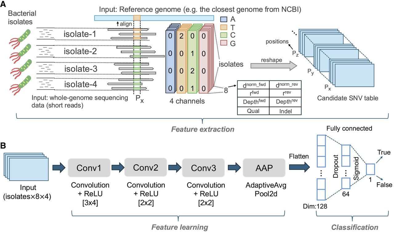
In this study, we curated real-world bacterial isolate WGS data (short reads) with manually labeled SNVs from prior studies conducted by our laboratory (Zhao et al. 2019; Conwill et al. 2022; Baker et al. 2025) to serve as training and validation data sets of AccuSNV. These data sets span three different species, with significantly different genome sizes and GC contents (Supplemental Table S2). We chose this data because, first, real-world data contain authentic sequencing noise, technical artifacts, and biological complexity that are difficult to simulate, providing a more robust foundation for model training compared to simulated data. Second, validated SNV data sets are rare, and most publicly available ones report only true positives without false SNVs, making it impossible for models to learn the features of false calls. Our laboratory's data sets overcome this limitation through manual labeling of both true and false SNVs, with standardized formats and stringent filtering (Supplemental Table S3). Third, for these data sets, pre-extracted alignment-derived features were already available, which greatly reduced the time and computational cost of model training because raw sequencing data did not need to be reprocessed. In addition, these curated features supported the quick generation of bar charts (Fig. 1) that visually distinguish high-quality from low-quality SNVs, providing an additional manual validation beyond automated filters (see Methods) and thereby enhancing label reliability. Fourth, the diversity of bacterial species and experimental contexts provides a foundation for generalization. Given these data sets, each candidate SNV site was encoded as a feature vector summarizing read-level signals and cross-sample alignment patterns (Fig. 2A), and a CNN was trained to classify them as true or false variants (Fig. 2B).
A deep learning framework that leverages across-sample comparisons for bacterial SNV calling. (A) Feature extraction pipeline: Short reads from bacterial isolates are aligned to a reference genome; features at candidate SNV positions are extracted across four channels (A, T, C, G). For each channel, there are eight features (for full details, see Supplemental Fig. S1): (Depthfwd, Depthrev) raw forward- and reverse-strand depths, (, ) forward- and reverse-strand normalized depths at each locus and each channel, (rfwd, rrev) forward- and reverse-strand relative depths showing the fraction of total coverage contributed by each isolate at each position and each channel, (Qual) consensus quality (FQ) scores produced by SAMtools, and (Indel) the number of reads supporting insertions and deletions at each position in that channel. These features are reshaped into a 4D (positions × isolates × features × channels) tensor and stored in a candidate SNV table for neural network input. (B) Model architecture: The input tensor is processed through three convolutional layers with ReLU activation and varying kernel sizes (shown in brackets), followed by adaptive average pooling. The output is then flattened and passed through fully connected layers with dropout for binary classification. The model finally outputs prediction probabilities, with SNVs classified as true if probabilities >0.5 and otherwise as false.
Critically, alignment error patterns, such as depth imbalances and mixed allelic signals in false positives, remain consistent across the three species used for training because false positives are primarily driven by common failure modes of short-read sequencing and alignment algorithms (Supplemental Fig. S2). This observation led us to hypothesize that a model could be built that effectively generalizes by learning these shared patterns.
The CNN model outperforms classical machine learning methods
To build AccuSNV, we first explored several classical machine learning models using the labeled SNV data set derived from read alignments of real bacterial sequencing data from the Lieberman laboratory. Input features (Supplemental Fig. S1) were constructed from read alignment patterns at candidate sites along with across-sample alignment statistics, and these were used to train XGBoost, random forest, support vector machines (SVM), and logistic regression models. We compared their performance against the CNN model with two and three convolutional layers to determine the optimal model complexity for capturing local sequence context and across-sample alignment patterns. To minimize bias, we randomly split the data set into training and validation sets five times, retrained all models on each split, and reported average performance metrics on the validation data (Supplemental Fig. S3).
The CNN model consistently achieved the highest scores across all evaluation metrics on the validation data set (Supplemental Fig. S3), outperforming all classical models (P < 0.05, Wilcoxon signed-rank test). Notably, the three-layer CNN also outperformed a shallower two-layer CNN architecture, demonstrating the importance of sufficient model depth for learning complex alignment patterns.
To understand which features contribute most to the CNN's performance, we conducted an ablation study by systematically removing different feature groups, retraining the model, and evaluating performance on the validation set (Supplemental Fig. S4). Consensus quality scores (Qual), derived from SAMtools FQ score, showed the largest impact when removed (0.66% F1 drop), consistent with their established importance in variant calling. However, removing any other single feature group resulted in modest performance decreases (<0.4% F1 drop), indicating that the CNN's robustness stems from integrating multiple complementary features rather than from relying on any single dominant signal.
The superior performance of CNN likely stems from fundamental architectural differences between CNN and classical machine learning approaches in handling genomic alignment data. Specifically, CNN preserves the relationship between alleles and their features across samples, whereas classical models require flattening to 2D vectors that lose crucial across-sample patterns. Additionally, CNNs can automatically learn complex patterns from the multidimensional alignment data and detect recurring motifs (e.g., the same minor allele across many samples) (Fig. 1B) regardless of their position in the tensor, whereas classical models rely on hand-crafted features and cannot capture these spatial relationships. These results motivated our choice of CNN with three convolutional layers as the core of the AccuSNV framework.
Overview of benchmark experiments
To evaluate the performance of AccuSNV, we benchmarked it against seven widely used SNV-calling tools (GATK v.4.5.0.0, FreeBayes v.1.3.6, SAMtools v.1.20, BactSNP v.1.1.0, VarScan v.2.4.6, breseq v.0.39.0, and Snippy v.4.6.0 [https://github.com/tseemann/snippy]) using both simulated and real-world data sets. The simulated data consisted of Illumina-like reads generated from six representative bacterial species across a range of sequencing depths (10× to 50×), divergence levels, and contamination scenarios, totaling thousands of samples. All tools were run using default or recommended parameters (see Supplemental Sec. 1). Across these diverse conditions, AccuSNV achieved consistently high accuracy, demonstrating robustness to challenges including low coverage, reference and genome divergence, and complex sequencing and alignment artifacts.
AccuSNV achieves high precision across sequencing depths
Sequencing depth serves as a critical factor influencing the accuracy of SNV calling, in which low coverage can lead to false positives or missed true SNVs (Fuchs et al. 2024). In this experiment, we simulated data sets of 10 isolates with sequencing depths of 10×, 20×, 30×, 40×, and 50× to compare the performance of different tools across varying sequencing depths. First, we selected six representative bacterial species (Cutibacterium acnes, Clostridium difficile, Escherichia coli, Klebsiella pneumoniae, Staphylococcus aureus, Streptococcus pneumoniae) and retrieved representative reference genomes (see Methods) from NCBI (Sayers et al. 2025). To mimic real-world scenarios, we simulated data sets of closely related organisms and a more distant reference genome. As illustrated in Supplemental Figure S5A, we introduced 1% SNVs and 500 indels into each reference genome with SimuG (Yue and Liti 2019) to create a root genome, which serves as the common ancestral sequence from which all simulated isolates will subsequently diverge. From this, we generated 10 mutant genomes (with about 70 mutant positions introduced per genome on average) per species with a phylogenetic structure intended to mimic realistic evolutionary relationships and simulated Illumina reads at 10× to 50× coverage using ART (Huang et al. 2012), resulting in 300 samples (10 isolates × 6 species × 5 depths). All reads were aligned back to the corresponding reference genome; SNV calling was performed using each tool; and precision, recall, and average F1 scores of each tool were calculated (Fig. 3).
AccuSNV achieves high precision across simulated data sets with different sequencing depths. Precision, recall, and average F1 scores of AccuSNV and seven other variant-calling tools were evaluated across simulated bacterial data sets at five sequencing depths (10×, 20×, 30×, 40×, and 50×). Axes use a transformed scale (−log10(1.0001 − x)) to enhance visualization in the higher range (0.9–1). Shapes represent species and colors represent tools. The vertical line at 0.99 precision highlights how more tools achieve high performance at greater sequencing depths. Top panels show precision–recall scatter plots for all tools and species at each depth. Middle panels provide a zoomed-in view of precision distributions across tools and species. Bottom panels summarize the average F1 score for each tool. The bar corresponding to AccuSNV is highlighted by a black outline.
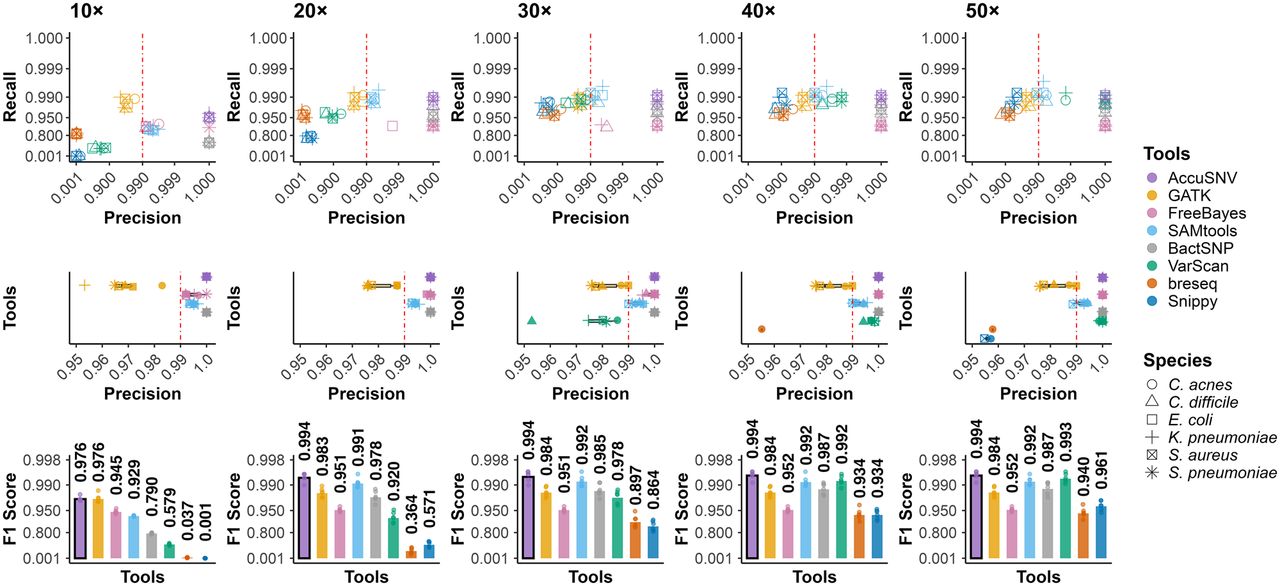
The performance of all tools improves with increasing sequencing depth, highlighting the importance of high-depth sequencing data for existing tools to accurately identify bacterial SNVs. In addition, AccuSNV achieves the highest average F1 score across all tested data sets (Fig. 3). In particular, AccuSNV achieves F1 scores of 97.6% and 99.4% at coverages as low as 10× and 20×, respectively, while maintaining 100% precision across all experiments. Among other tools, BactSNP also achieves perfect precision but with lower recall compared with AccuSNV. At a sequencing depth of 10×, GATK has higher recall than AccuSNV, but its average precision is 96.8% compared with 100% for AccuSNV. SAMtools and VarScan perform competitively at higher depths but underperform at 10×, with F1 scores dropping to 92.9% and 57.9%, respectively. The remaining three tools, FreeBayes, breseq, and Snippy show poorer performance compared with other tested tools across all data sets. The performance of both breseq and Snippy drop markedly at 10× depth, because the conservative filters, such as minimum depth, allele-fraction and strand-balance requirements, and evidence-count thresholds, discard many true variants and true reference calls once the effective coverage falls below these cutoffs.
AccuSNV maintains high accuracy on large and noisy simulated data sets
In real-world scenarios, sequencing samples from different isolates often have varying depths and complex phylogenetic relationships. Moreover, previous studies have shown that the divergence between the target genome and the reference genome significantly impacts bacterial SNV-calling performance (Bush et al. 2020). Lastly, many real-world data sets contain large isolate collections, introducing additional complexity to SNV detection. To better reflect these real-world challenges, we generated an additional large-scale, noisy simulated data set for evaluation. Notably, FreeBayes and breseq were excluded from this experiment and subsequent real-world data evaluations owing to their lower accuracy in earlier evaluations and substantially longer runtimes (Supplemental Table S1).
To investigate the influence of the reference genome, we first generated four root genomes per species of varying reference divergence from the reference genome. From each root genome, we simulated a phylogenetic tree with 100 strains using Msprime (Baumdicker et al. 2022), which provided the number of mutations along each branch for the given mutation rate (5 × 10⁻¹⁰ here). We then assigned 80% of the mutations as SNVs and 20% as indels and used SimuG to generate the corresponding mutated genomes. We focused solely on SNVs and indels without larger recombination or rearrangement events, as this analysis targets very closely related isolates in which such structural variations are rare. Paired-end reads were simulated at random depths between 15× and 70×. In total, this yielded 2400 samples (100 isolates × six species × four reference divergence levels) for evaluating SNV-calling tools (Supplemental Fig. S5B).
AccuSNV exhibits the most competitive performance among all tested tools, with average F1 scores exceeding 99% across all data sets (Fig. 4). It maintains perfect precision across all reference divergence levels and achieves an F1 score >99.1% even at the highest reference divergence (1%). In contrast, other tools show greater variability: VarScan, SAMtools, and Snippy all experience significant drops in precision or recall at higher reference divergence levels. Although GATK performs comparably to, or slightly better than, AccuSNV at the 0.05% and 0.1% reference divergence levels in terms of F1 score, this is driven by increased recall at the cost of reduced precision, which is suboptimal when comparing closely related genomes in which precision is critical (Bush 2021). BactSNP also maintains perfect precision across all data sets but with consistently lower recall, leading to reduced F1 scores, especially under higher reference divergence.
AccuSNV maintains high accuracy on large and noisy simulated data sets. Performance comparison of six SNV-calling tools across four reference divergence levels. Axes use a transformed scale (−log10(1.0001 − x)) to enhance visualization in the higher range (0.9 to one). Shapes represent species, and colors represent tools. Panels show average recall (top), precision (middle), and F1 score (bottom) across all species. AccuSNV bars are highlighted with a black outline.
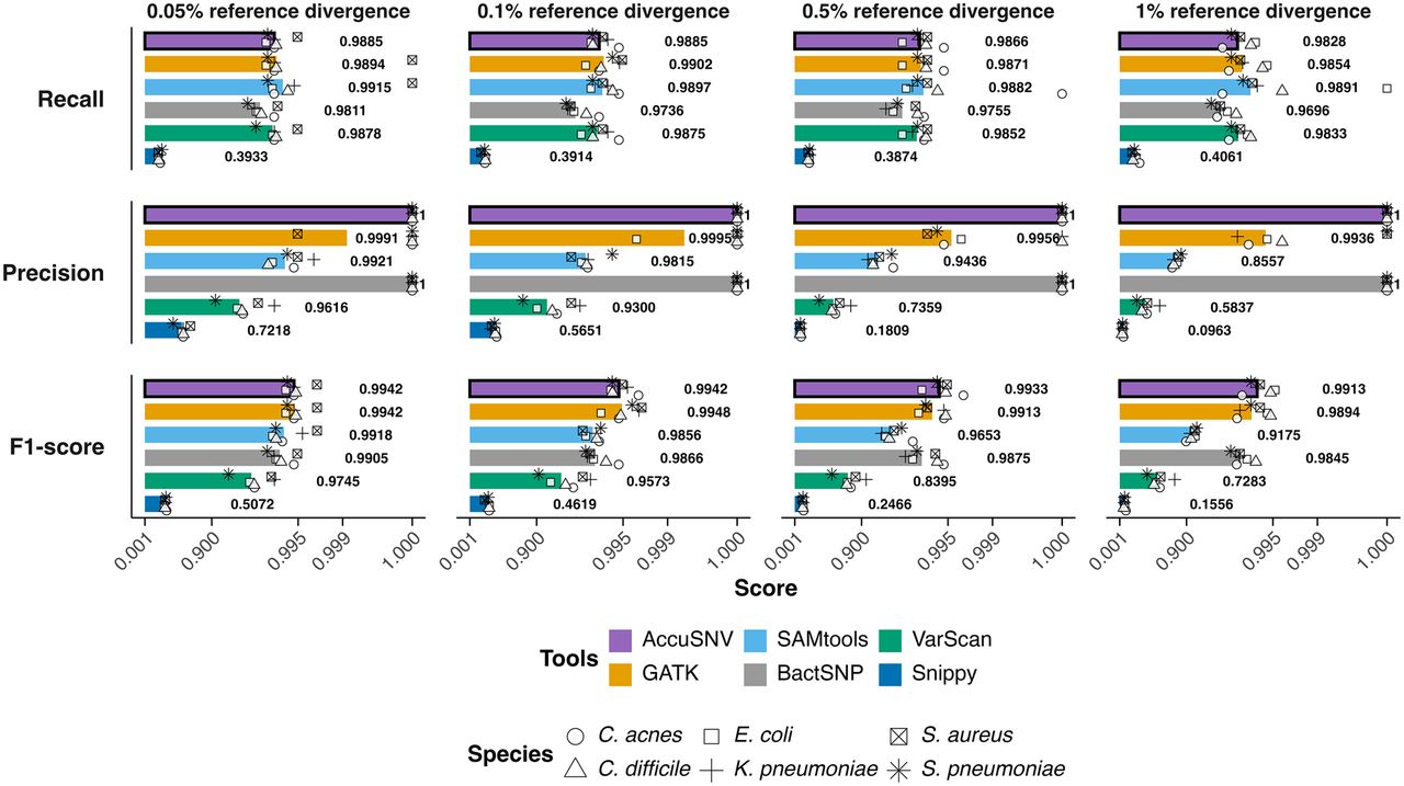
Overall, all tools exhibit decreased performance as the divergence between the root genome and the reference genome increases, highlighting the growing difficulty of variant calling when read–reference mismatches become more prevalent. Despite this, AccuSNV shows minimal performance fluctuation across reference divergence levels. In addition, tools such as SAMtools and VarScan, which performed well in the previous experiments with only 10 strains at 50×, uniform sequencing depth, and simplified phylogenetic structure, showed markedly reduced performance on this more realistic and noisy data set. The performance degradation is particularly pronounced for Snippy, which is sensitive to false-positive calls under increased reference divergence and noise owing to misalignments near indels and other structural differences (Supplemental Fig. S6; Yoshimura et al. 2019). These results indicate that the robustness of existing tools may decline under more complex and realistic sequencing conditions. In contrast, AccuSNV maintains both high accuracy and consistency, supporting its use in large-scale bacterial variant detection across diverse and complex conditions.
Although the experiment with varying sequencing depths reflects the realistic heterogeneity commonly observed in bacterial genomics studies, using a uniform sequencing depth allows us to examine the effect of reference divergence without the confounding effect of sequencing depth. We therefore conducted an additional controlled experiment with a uniform sequencing depth of 50× across all isolates to disentangle the impact of reference divergence from depth variation (Supplemental Fig. S7). Under this controlled setting, AccuSNV maintains top-tier performance across all reference divergence levels (0.05%–1%), still achieving F1 scores >99.1% with perfect precision even at 1% divergence.
Experiments on highly variable isolates
Some real-world bacterial populations, such as those from environmental samples, can exhibit substantial genetic variability between isolates. To evaluate how well different tools perform under such conditions, we varied the mutation rate in 100 Escherichia coli genomes using Msprime (see Supplemental Fig. S5B), based on a root genome containing 1% sequence variation. Specifically, we tested mutation rates of 5 × 10⁻⁹, 5 × 10⁻⁸, and 1 × 10⁻⁷, along with the original rate of 5 × 10⁻¹⁰ per site per generation. We reran all tools on these data sets and recorded the results (Supplemental Fig. S8).
As mutation rates increased, all tools exhibited more false positives and false negatives. Nevertheless, AccuSNV achieved a high average F1 score (98.85%) by balancing recall and precision. GATK (with 98.81% average F1 score) showed the most competitive F1 score at higher mutation rates but had lower precision compared with AccuSNV. In contrast, BactSNP (with 98.11% average F1 score) maintained higher precision across all data sets, but its recall was substantially lower. SAMtools (with 98.33% average F1 score) achieved the best recall across all data sets, yet it produced more false positives at higher mutation rates. Overall, AccuSNV demonstrated a highly robust and reliable performance across mutation rates, underscoring its effectiveness for analyzing highly variable bacterial isolates.
Computational efficiency comparison
To compare the running time and memory usage of different tools, we applied all tools to 10-strain and 100-strain E. coli simulated data sets and recorded the computational performance metrics (Supplemental Table S1). AccuSNV demonstrated competitive efficiency, completing analysis in 30.3 min for 10 isolates (50×) and 64.5 min for 100 isolates (15×–70×), with memory usage of 1140 MB and 1340 MB, respectively. Although some tools like Snippy showed faster execution times (5 min on a 10-strain data set and 50 min on a 100-strain data set), AccuSNV maintained better performance without the extreme computational demands observed in tools like FreeBayes and breseq, which failed to complete within reasonable time limits on the larger data set (running >2 days on the 100-strain data set). The results demonstrate that AccuSNV provides a balance between accuracy and computational efficiency for bacterial SNV-calling applications.
AccuSNV shows good robustness in simulated contaminated samples
To assess the robustness of SNV-calling tools under contamination, we simulated data sets with increasing levels of contamination, either from other strains of the same species or from closely related species, under both high and low sequencing depths. AccuSNV consistently achieved higher F1 scores compared with other tools in low-depth contaminated data sets and maintained perfect precision in all tested data sets. In high-depth settings (50× depth) with contamination from both other strains and closely related species, VarScan achieved the highest F1 scores across all data sets, with AccuSNV ranking second owing to slightly lower recall. However, in this high-depth setting, when contamination originated from closely related species, VarScan exhibited reduced precision compared with AccuSNV. Full results are provided in Supplemental Section 2.1 and Supplemental Figures S9–S12.
AccuSNV demonstrates high accuracy on real-world test data
Real-world data from independent studies, featuring diverse sequencing protocols, depths, species, and collection contexts, offer a more rigorous assessment for evaluating the robustness and accuracy in practical applications, as simulations rarely include all types of error and variability in the real world. In this experiment, we evaluated AccuSNV and other tools using four publicly available bacterial sequencing data sets (Snitkin et al. 2012; Kim et al. 2014; Giulieri et al. 2022; Buddle et al. 2024), each derived from a distinct study/author group and accompanied by manually curated and reported SNVs that underwent careful quality control (QC) rather than being taken directly from automated tool outputs. The four data sets differ in read types (single-end vs. paired-end), bacterial species, and isolate numbers (Supplemental Fig. S13). The data set from Snitkin et al. (2012) comprises single-end reads from a hospital outbreak of K. pneumoniae, whereas the others involve paired-end sequencing of S. aureus or C. difficile collected under varying evolutionary or clinical contexts. These differences in sequencing protocols, strain diversity, and sampling settings create a heterogeneous and realistic benchmark for evaluating SNV-calling accuracy and robustness.
All tools called distinct sets of SNVs across these data sets, with none matching the reported SNVs exactly (Fig. 5). Across all four data sets, AccuSNV demonstrates strong concordance with reported SNVs while minimizing tool-specific SNVs unsupported by other methods or the original studies (only 110 unreported SNVs compared with 127–422 for other tools, except Snippy, which had 26 but identified much fewer reported SNVs).
AccuSNV demonstrates high accuracy and precision on additional real-world bacterial sequencing data sets. We evaluated SNV concordance between AccuSNV and five other tools across four published bacterial data sets with curated SNVs (Supplemental Fig. S13). UpSet plots (center) display the SNVs overlap count of tool-identified SNVs and reported SNVs. The red-outlined dash box highlights a group of four SNVs identified by all tools except AccuSNV and the original study (corresponding IGV screenshot is shown in the top right panel) (Robinson et al. 2011). The IGV screenshot includes two sample tracks, one carrying the reference allele and one carrying the alternative allele, with the variant position highlighted by a red box. Red reads indicate an inferred insert size larger than expected, which may suggest the presence of a deletion or a possible alignment artifact. The bottom panels display IGV screenshots of five unique SNVs identified by other methods but not supported by AccuSNV or the original study. The colored borders around each IGV screenshot correspond to the dashed boxes in the UpSet plot, indicating the group from which each SNV originated. Below each IGV screenshot is a description of the source of errors, highlighting typical error signatures such as misalignments near large structural variants, indels, and paralogous alignments (as reported by Koboldt 2020). We note that these error modes are not generally tool specific but that these tool-specific SNVs happen to have these error modes. Also see Supplemental Figures S14–S17.
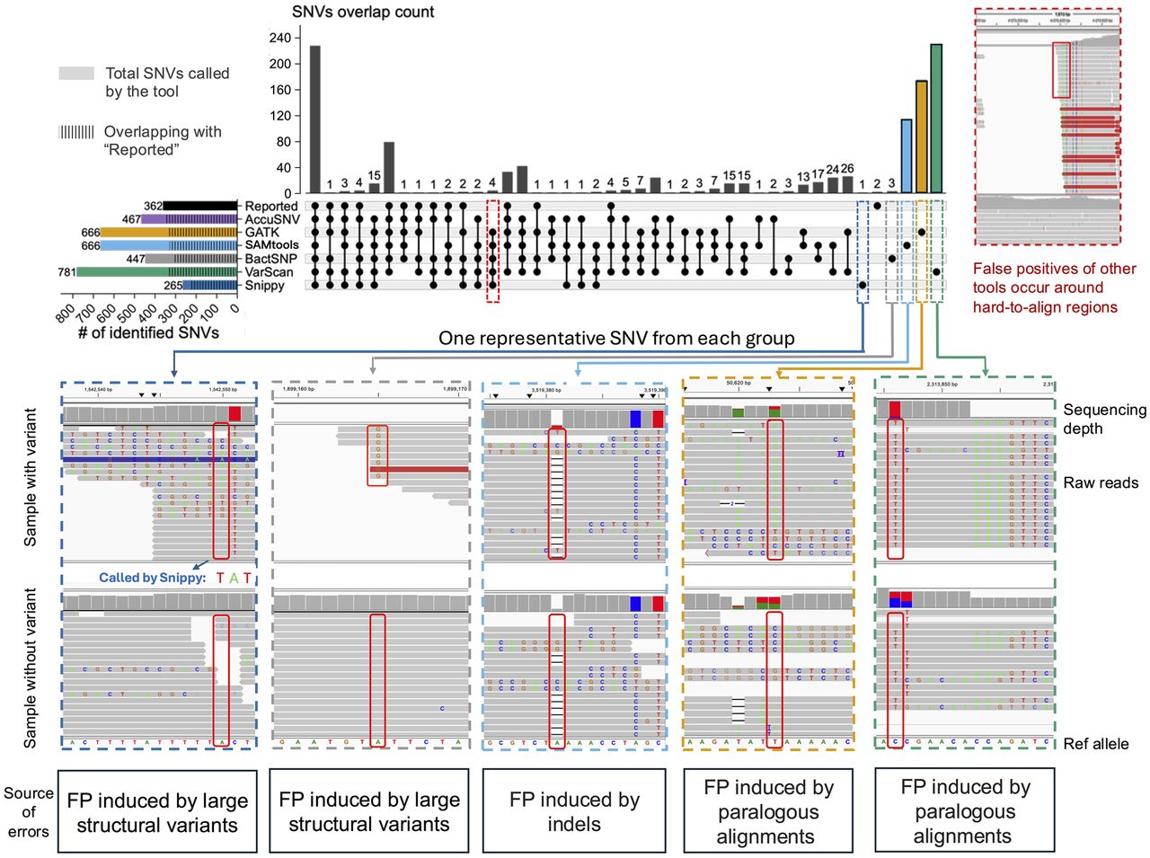
Inspection of discordances among SNV-calling methods illustrates that AccuSNV avoids false positives called by other tools, generally caused by alignment errors. For example, a notable group of SNVs is highlighted in the red dashed box (Fig. 5); these four SNVs from the same study were called by all other tools but not called by AccuSNV or the original study. To investigate the basis of this discrepancy, we visualized the corresponding BAM files of these four SNVs, one of which is shown in the panel outlined on the right. These four SNVs appear to be false positives located in hard-to-align regions, owing to divergent regions between the sample and reference.
In addition, all tools except AccuSNV reported unique SNVs that were not supported by any other method or the original study. To further examine these unique SNVs, we manually reviewed five random, unique SNVs from tested tools and visualized their read alignments (Fig. 5, bottom panels). In all cases, the alignments revealed problematic mapping features, such as soft clipping, inconsistent base support, or alignment gaps. These findings suggest that these unique SNVs called by other tools are false positives resulting from alignment errors. This observation agrees with previous studies, such as the one by Koboldt (2020), which identified similar artifacts in short-read alignments, leading to false-positive variant calls. Although the IGV examples in Figure 5 highlight representative alignment-related error modes, we further assessed whether these patterns generalize across data sets by quantifying site-level signatures associated with reported and unique SNVs for each variant caller. We observed that across four real-world data sets, different callers exhibit distinct but data set–dependent distributions of allele balance, sequencing depth, and mapping quality (Supplemental Figs. S14–S17). These results indicate that although certain error modes recur, their quantitative manifestations vary substantially across data sets, complicating the use of universal hard filtering thresholds. In contrast, AccuSNV is able to filter these false positives by capturing informative across-sample features from alignment data rather than relying on manually defined thresholds or manual filtering of individual positions.
Output and downstream analysis modules of AccuSNV
To support users with varying levels of computational expertise, AccuSNV offers comprehensive output and downstream analysis modules based on the identified SNVs. The core output includes a compressed SNV table in NumPy's NPZ format (a compact binary file for storing arrays), a human-readable tab-separated summary of all the SNVs (TSV) including the allele call for each sample, a graphical HTML report, and a set of QC figures (Fig. 6).
Output and downstream analysis modules of AccuSNV. The core outputs include (1) a compressed SNV table in NumPy's NPZ format storing detailed feature vectors and prediction scores; (2) a human-readable text summary file (TSV) listing all identified SNVs with key attributes; (3) a set of quality control (QC) figures summarizing read coverage, base calls, mapping quality scores, etc.; and (4) a HTML report that integrates summary tables and bar charts of identified variants. Homoplasic SNVs in the figure refers to variants in which the same derived nucleotide arises independently in two or more lineages since their divergence from a common ancestor with a different ancestral base. These SNVs can be used to infer parallel, convergent, or revertant evolutionary events (Edwards et al. 2021).
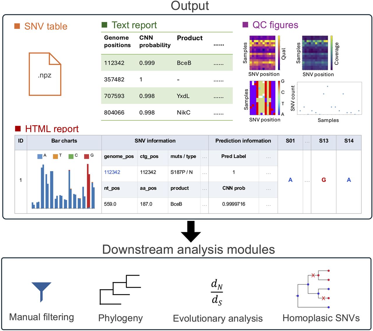
The HTML report provides an interactive platform for variant review. Each predicted SNV is visualized with a bar chart showing allele frequency distributions across isolates (as in Fig. 1), alongside detailed metadata such as strand-specific depth, mapping quality statistics, and various filter flags. A demo output HTML report can be found at GitHub (https://heruiliao.github.io/). This design helps users assess variant confidence and identify potentially ambiguous cases that may require manual curation. In addition, AccuSNV generates multiple QC figures to assist in data quality assessment, including heatmaps of genome coverage and allele count distributions across samples. The human-readable tab-separated TSV file presents essential information for each SNV for rapid inspection and integration with external pipelines. Lastly, the compressed SNV Numpy table stores all variant-level features and prediction outputs in an efficient binary format, which serves as input for downstream modules.
To facilitate related applications, AccuSNV includes built-in modules for common downstream analyses. These modules enable manual filtering, phylogenetic tree construction, calculation of dN/dS ratios to assess selective pressures, and identification of homoplasic SNVs (Edwards et al. 2021). Additionally, users can export filtered variants for phylogenetic analysis with external tools.
Together, these outputs and utilities make AccuSNV a versatile and accessible tool for high-confidence bacterial SNV detection and interpretation.
Discussion
In this study, we present AccuSNV, a deep learning–based variant-calling framework designed for high-precision SNV detection from bacterial WGS data. By encoding multisample read alignment data into structured feature vectors and leveraging a CNN, AccuSNV effectively captures across-sample patterns that are often ignored by conventional methods. Our approach addresses key challenges in bacterial variant calling, including low sequencing depth, high intraspecies diversity, and genome complexity. As a result, AccuSNV enables accurate bacterial SNV calling for users with varying levels of expertise, without the need for hard-coded thresholds or extensive manual filtering. Although a few tools occasionally achieved comparable or better performance under specific conditions, AccuSNV was consistently the best or among the top-performing methods across all sequencing depths, reference and sequence divergence levels, and contamination scenarios (Figs. 3Figure 4.–5), demonstrating its broad applicability and scalability for bacterial genomics research. Interestingly, GATK performed as or nearly as well as AccuSNV under many conditions with default parameters on simulated data, likely because of its integration of across-sample comparisons (Figs. 3, 4), but still had more identified false positives when challenged with real-world data (Fig. 5), likely owing to structural variations between the reference and real samples. We note that all the tested pipelines can yield reliable results in many applied studies, particularly when users manually tune parameters, apply additional post hoc filtering, or visually inspect alignments, especially for high-depth data sets with closely related references. However, this reliance on data set–specific decisions and expert judgment can limit reproducibility and scalability across large or heterogeneous cohorts, in which systematic alignment-related error modes become more prominent (Yoshimura et al. 2019). AccuSNV minimizes manual parameter tuning by learning to identify false-positive SNVs directly from across-sample alignment patterns, enabling consistent performance across sequencing depths and reference divergence levels. Feature ablation analysis revealed that this robustness arises from integrating multiple complementary features rather than depending on any single signal, allowing the CNN to adapt to diverse sequencing conditions (Supplemental Fig. S4).
Despite these advances, AccuSNV has several limitations. First, the current implementation is designed and trained specifically for short-read sequencing data. Extending AccuSNV to long-read sequencing platforms such as Oxford Nanopore Technologies (ONT) or Pacific Biosciences (PacBio) would require retraining on platform-specific data sets and potentially incorporating features that capture their distinct error profiles. Second, misclassifications may still arise in extremely challenging or ambiguous cases encountered in real-world data, especially those involving false-positive SNVs arising from an error mode not represented in the training set. For example, although the training and test species span a broad range of genome sizes and GC content commonly observed in bacterial pathogens and commensals (Supplemental Table S2), AccuSNV has not yet been evaluated on bacteria with extreme genomic features (e.g., GC content <20% or >70%) or other haploid organisms such as yeast. To enable users to evaluate AccuSNV's performance on new use cases, AccuSNV provides an interactive HTML report and multiple QC visualizations that allow users to inspect candidate SNVs and flag potential false positives for downstream curation. Third, AccuSNV is specifically designed for SNV calling and does not currently support the identification of structural variants (SVs), such as insertions, deletions, or inversions. Fourth, the method is not directly applicable to metagenomic data sets, in which a single sample may contain multiple closely related strains, resulting in more complex and ambiguous alignment patterns than those encountered in isolate-based WGS. Finally, although the across-sample alignment patterns that AccuSNV leverages to identify false positives may be consistent across organism types, the current implementation is limited to haploid genomes. Diploid genomes present a fundamentally different classification problem: distinguishing true heterozygous variants from sequencing or alignment errors, rather than simply identifying sites that deviate from a single reference allele.
We note that in all of our evaluation experiments, we assess each genomic position as either a true or false variant site rather than evaluating individual per-sample variant calls. Thus, many individual false calls are reduced to only a single count in our evaluations. In practical applications, especially under low coverage or high reference divergence, many samples may have false positives or false negatives at a single position. As such, the position-level evaluation presented here provides a conservative benchmark of tool performance in these noisy and complex scenarios.
Looking forward, several directions can extend the utility of AccuSNV. One promising avenue is to expand the framework to support small indel detection by incorporating indel-aware features and labels during model training. Another direction is to explore whether across-sample alignment patterns in metagenomic data can be modeled to distinguish strain-specific SNVs, potentially enabling AccuSNV to operate in complex microbial communities. Extending the approach to diploid genomes is another promising direction that would require incorporating heterozygosity-aware features and training on data sets with appropriately labeled homozygous and heterozygous variants. However, these efforts may be constrained by the limited availability of real-world data sets with manually validated labels.
In conclusion, by reducing the need for manual thresholding and incorporating interpretable QCs, AccuSNV makes high-confidence bacterial SNV calling accessible to users with varying levels of computational expertise. This accessibility makes it particularly well suited for studies of within-microbiome evolution, large-scale evolution experiments, and bacterial epidemiology, even when working with low-coverage or noisy sequencing data. By lowering technical barriers, AccuSNV enables broader adoption of high-precision SNV calling in diverse research and clinical settings.
Methods
Overview of AccuSNV
AccuSNV is designed for high-precision SNV calling from WGS data of bacterial isolates. It takes a reference genome and WGS short-read data from multiple bacterial samples (isolates) as input, and outputs identified SNVs along with associated information such as annotations, predicted probabilities, and visualization results, etc. (Figs. 2, 6). AccuSNV leverages deep learning to distinguish true variants from sequencing or mapping artifacts, eliminating the need for manual filtering. Specifically, to address challenges such as low sequencing depth, genomic intraspecies diversity, variability in sample size, and sequencing quality across data sets, AccuSNV employs a CNN-based framework to learn informative patterns from multisample read alignment data. Here, we chose CNN for its ability to extract local features and maintain translation invariance (Lecun et al. 1998), which enables the robust detection of across-sample patterns from diverse and noisy bacterial isolate alignments. To implement this CNN-based approach, AccuSNV first identifies candidate SNV sites using SAMtools and extracts read-level features from bacterial isolate alignments using a Snakemake-based pipeline (Fig. 2A), including read orientation, read counting, mapping quality score, etc. (Supplemental Fig. S1). These features are converted into a four-dimensional numerical feature vector, allowing the CNN to better capture both local and across-sample patterns. The CNN model (Fig. 2B) was trained using these four-dimensional feature vectors as input, and the final pretrained model is provided to perform binary SNV classification on new data sets.
Reference genomes used in this study
C. acnes C1 (GCF_000302515.1), C. difficile R20291 (GCF_000027105.1), E. coli str. K-12 substr. MG1655 (GCF_000005845.2), K. pneumoniae subsp. pneumoniae NTUH-K2044 (GCF_000009885.1), S. aureus subsp. aureus NCTC 8325 (GCF_000013425.1), and S. pneumoniae R6 (GCF_000007045.1) genomes were obtained from the NCBI Genomes database (https://www.ncbi.nlm.nih.gov/home/genomes/) and selected as reference genomes in this study.
Training and validation data sets
To train and evaluate the model, we collected a total of 7638 “quality-filtered” SNVs (labeled as “true”) from 5432 isolates from three data sets published in previous studies (Zhao et al. 2019; Conwill et al. 2022; Baker et al. 2025) conducted by our laboratory and 6306 “low-quality” SNVs filtered out during processing for these studies (labeled as “false”). These data sets comprise 222 lineages (finely resolved clades separated by fewer than 100 mutations across the core genome) (Conwill et al. 2022; Baker et al. 2025) and include carefully curated SNVs based on extensive manual validation of filters in a study-specific manner. The criteria used in each study to define “quality-filtered” SNVs are summarized in Supplemental Table S3. To verify the collected positions in the training data, we randomly picked up to 10 true and 10 false positions per lineage (for a maximum of 20 per lineage), but some lineages contained fewer than 20 available sites, resulting in 2859 positions that were manually inspected using generated bar charts (see example in Fig. 1). These bar charts are available at Zenodo (https://zenodo.org/records/17058222). Manual inspection confirmed that the assigned labels were accurate and consistent with the expected patterns. These data were split into training and validation sets at a four:one ratio, stratified by lineages across the three data sets. This ensured that the validation set contained isolates from different lineages and data sets, resulting in 10,887 SNVs for training and 3057 SNVs for validation and thereby improving the generalizability of the trained model. Accession numbers and additional details regarding the training data are provided in Supplemental Table S4. Additionally, to assess tool performance on real-world data from independent studies, we collected 362 reported SNVs from four different published data sets, in which SNVs had been carefully validated in the original studies through stringent filtering and manual inspection rather than taken directly from automated tool outputs. Detailed information on all seven data sets is provided in Table 1.
Summary of the seven real bacterial whole-genome sequencing data sets used in this study
| Type/data set ID | Species | No. of lineages | No. of isolates | No. of true SNVs | No. of false SNVs | Source |
|---|---|---|---|---|---|---|
| Training/validation | ||||||
| Zhao_2019 | B. fragilis | 11 | 556 | 227 | 492 | (Zhao et al. 2019) |
| Conwill_2022 | C. acnes | 50 | 854 | 1972 | 3840 | (Conwill et al. 2022) |
| Baker_2025 | C. acnes | 85 | 2007 | 3444 | 554 | (Baker et al. 2025) |
| S. epidermidis | 76 | 2015 | 1995 | 1420 | ||
| Test | ||||||
| Kim_2014 | S. aureus | 1 | 121 | 265 | — | (Kim et al. 2014) |
| Buddle_2024 | C. difficile | 1 | 96 | 55 | — | (Buddle et al. 2024) |
| Snitkin_2012 | K. pneumoniae | 1 | 20 | 31 | — | (Snitkin et al. 2012) |
| Giulieri_2022 | S. aureus | 1 | 16 | 11 | — | (Giulieri et al. 2022) |
Identification of candidate SNVs
To identify candidate SNV sites from raw sequencing data, we implement a modular pipeline built with Snakemake (Mölder et al. 2021). The process begins with quality trimming of reads using cutadapt (v.1.18) (Martin 2011) and Sickle (v.1.33; -g -q 20 -l 50 -x -n; https://github.com/najoshi/sickle) followed by reference-based alignment via BWA-MEM (v.0.7.18) (Li and Durbin 2009). Aligned reads are converted to sorted and indexed BAM files. SAMtools markdup (v.1.21.1; -r -s -d 100 -m s) is used to remove duplicate reads from each sample. Pileup and VCF files are then generated using SAMtools (Li et al. 2009) mpileup (v.1.21.1; -q30 -x -s -O -d3000) and BCFtools (Danecek et al. 2021) view (v.1.21.1; -Oz -v snps -q .75). Critically, AccuSNV leverages Snakemake's workflow management to automatically handle task dependencies and enable parallel execution of independent, sample-level preprocessing steps across multiple cores or cluster nodes when resources are available. This parallel execution strategy substantially reduces computational time compared with sequential preprocessing approaches, particularly for large data sets. As a result, although runtime scales approximately linearly with data set size for tools that require predominantly sequential preprocessing (e.g., GATK), AccuSNV maintains efficient performance when scaling tens to hundreds of isolates (Supplemental Table S1).
For each input sample, preliminary SNVs are extracted from VCF files and saved in compressed intermediate files. Then, the pipeline aggregates variant positions across all samples and combines these positions with alignment-derived metrics, such as read counting and mapping quality score, into a candidate mutation table using custom Python scripts. This table contains informative alignment statistics for each candidate SNV and serves as the input for downstream analysis.
Feature extraction
To ensure the CNN can effectively capture informative patterns across bacterial isolates, AccuSNV transforms raw alignment data into structured four-dimensional feature vectors. Specifically, for each candidate SNV position, we aggregate information from all reads supporting each allele in each sample, including base counts on forward and reverse strands, mapping quality scores, and indel signals (the number of reads supporting insertions and deletions, broadcast across the four base channels per sample) (Supplemental Fig. S1). Notably, these features were selected because they are commonly used in the manual filtering step across previous studies (Zhao et al. 2019; Conwill et al. 2022; Key et al. 2023) for distinguishing “quality-filtered” SNVs from “low-quality” positions. In addition, we incorporate two normalized coverage-based features, and ri,j, to better represent both across-position and across-sample variation. These two features are computed separately for forward and reverse strands to retain strand-specific information:
During feature extraction, we further observed that certain low-quality positions display extremely unbalanced coverage distributions, in which the depth of the putative minor allele is orders of magnitude lower than that of the major allele (see Supplemental Fig. S18). Such unusual “gap cases” are underrepresented in the training data and tend to be misclassified by the CNN. To ensure these extreme cases are consistently represented, we introduced a normalization-based adjustment in the feature encoding step, implemented through a Z-score framework:
These features are then encoded as a four-dimensional feature vector (Fig. 2), in which the last dimension represents the nucleotide channels. This four-dimensional feature encoding has two key advantages over traditional feature representation like raw VCF statistics or flattened alignment matrices. First, it encodes comprehensive alignment features in a structured, image-like format that is well suited for the CNN model, enabling it to leverage translation invariance and local feature extraction. Second, it preserves across-sample information, enabling the model to capture shared or contrasting patterns among isolates at each site. These patterns are not accessible to conventional single-sample variant callers but are essential for distinguishing true SNVs from sequencing or alignment artifacts.
Deep learning framework
Given the extracted feature vectors, we employ a CNN to classify the candidate SNVs. There are two major challenges in applying CNN to this task. First, the number of bacterial isolates varies across data sets, leading to input tensors with different dimensions along the sample axis. Such variability poses a problem for standard CNN architectures, which require fixed input dimensions for training and inference. Second, compared with natural image tensors that often contain rich spatial information and high-dimensional features, our input tensors have a much lower feature dimensionality. Commonly used deep or parameter-heavy models are therefore prone to overfitting, especially given the limited number of labeled training examples.
To address these issues, we designed a CNN architecture to accommodate the varying alignment data. The model consists of convolutional, pooling, and fully connected layers (Fig. 2B). Specifically, we used three convolutional layers to hierarchically capture both localized signal structures and broader across-sample patterns. These three layers use 32, 64, and 128 filters with kernel sizes of 3 × 4, 2 × 2, and 2 × 2, respectively. Each convolutional layer is followed by a ReLU activation function. To accommodate inputs with variable sample sizes, we apply an adaptive average pooling operation (Hsin and Su 2021) along the sample axis, compressing variable-length inputs into a fixed-size representation. Unlike standard pooling layers with fixed kernel sizes, adaptive pooling dynamically divides the input into regions such that the output always has the same predefined shape, regardless of the input size. Let the X ∈ ℝx×y×z×4 be the input feature vector, where x is the number of candidate SNV postions, y is the number of samples (bacterial isolates), z is the number of features, and 4 is the input channels. Then, the output tensor Z of the adaptive average pooling layer is
Model training
The model was trained using real-world bacterial WGS data with curated labels obtained from previously published studies (Zhao et al. 2019; Conwill et al. 2022; Baker et al. 2025), as summarized in Table 1. During training, the binary cross-entropy loss function was used as the objective function.
Evaluation metrics
To evaluate the performance of different tools, we used five standard metrics: accuracy, precision, recall, F1 score, and area under the curve (AUC). Let TP, FP, TN, and FN denote the number of true positives, false positives, true negatives, and false negatives, respectively. The evaluation metrics are defined as
Data sets
Real-world data sets used in this paper are all publicly available. Bar charts for the 2859 positions selected for manual label inspection are available at Zenodo (https://zenodo.org/records/17058222) and in the Supplemental Data. A demo output HTML report of AccuSNV can be found at GitHub (https://heruiliao.github.io/).
Code availability
The source code of AccuSNV is freely available at GitHub (https://github.com/liaoherui/AccuSNV) and as Supplemental Code. AccuSNV is also available via Bioconda at https://anaconda.org/bioconda/accusnv. The command lines for running other SNV-calling tools are provided in the Supplemental Methods. The custom scripts necessary to reproduce the benchmarking experiments can be accessed at GitHub (https://github.com/liaoherui/accusnv-eval) and as Supplemental Code.
Competing interest statement
The authors declare no competing interests.
Acknowledgments
This work has been supported by MIT-Novo Nordisk artificial intelligence postdoctoral fellowship to H.L. and National Institutes of Health grants 1DP2GM140922 and R35GM156282 to T.D.L. I.L.-M., M.F., and F.M.K. were supported by the Max Planck Society. During the preparation of this work, the authors used ChatGPT (https://chatgpt.com/) in order to rephrase sentences. We thank members of the Lieberman laboratory and Key laboratory for helpful comments.
Author contributions: Methodology was by H.L., P.T., A.C., E.B.Q., A.H.M., J.S.B., M.F., I.L.-M., F.M.K., and T.D.L. Investigation was by H.L., A.H.M., T.D.L., and L.R.B. Funding acquisition was by H.L. and T.D.L. Writing was by H.L. and T.D.L.
Footnotes
[1] Supplementary material [Supplemental material is available for this article.]
[2] Article published online before print. Article, supplemental material, and publication date are at https://www.genome.org/cgi/doi/10.1101/gr.281341.125.
[3] Freely available online through the Genome Research Open Access option.
References
- ↵Ahmed SF, Alam MSB, Rozbu MR, Ishtiak T, Rafa N, Mofijur M, Shawkat Ali ABM, Gandomi AH. 2023. Deep learning modelling techniques: current progress, applications, advantages, and challenges. Artif Intell Rev 56: 13521–13617. 10.1007/s10462-023-10466-8
- ↵Baker JS, Qu E, Mancuso CP, Tripp AD, Conwill A, Lieberman TD. 2025. Intraspecies dynamics underlie the apparent stability of two important skin microbiome species. Cell Host Microbe 33: 643–656. 10.1016/j.chom.2025.04.010
- ↵Barrick JE, Yu DS, Yoon SH, Jeong H, Oh TK, Schneider D, Lenski RE, Kim JF. 2009. Genome evolution and adaptation in a long-term experiment with Escherichia coli. Nature 461: 1243–1247. 10.1038/nature08480
- ↵Barrick JE, Colburn G, Deatherage DE, Traverse CC, Strand MD, Borges JJ, Knoester DB, Reba A, Meyer AG. 2014. Identifying structural variation in haploid microbial genomes from short-read resequencing data using breseq. BMC Genomics 15: 1039. 10.1186/1471-2164-15-1039
- ↵Baumdicker F, Bisschop G, Goldstein D, Gower G, Ragsdale AP, Tsambos G, Zhu S, Eldon B, Ellerman EC, Galloway JG, 2022. Efficient ancestry and mutation simulation with msprime 1.0. Genetics 220: iyab229. 10.1093/genetics/iyab229
- ↵Buddle JE, Thompson LM, Williams AS, Wright RCT, Durham WM, Turner CE, Chaudhuri RR, Brockhurst MA, Fagan RP. 2024. Identification of pathways to high-level vancomycin resistance in Clostridioides difficile that incur high fitness costs in key pathogenicity traits. PLoS Biol 22: e3002741. 10.1371/journal.pbio.3002741
- ↵Bush SJ. 2021. Generalizable characteristics of false-positive bacterial variant calls. Microbial Genomics 7: 000615. 10.1099/mgen.0.000615
- ↵Bush SJ, Foster D, Eyre DW, Clark EL, De Maio N, Shaw LP, Stoesser N, Peto TEA, Crook DW, Walker AS. 2020. Genomic diversity affects the accuracy of bacterial single-nucleotide polymorphism–calling pipelines. GigaScience 9: giaa007. 10.1093/gigascience/giaa007
- ↵Conwill A, Kuan AC, Damerla R, Poret AJ, Baker JS, Tripp AD, Alm EJ, Lieberman TD. 2022. Anatomy promotes neutral coexistence of strains in the human skin microbiome. Cell Host Microbe 30: 171–182.e7. 10.1016/j.chom.2021.12.007
- ↵Danecek P, Bonfield JK, Liddle J, Marshall J, Ohan V, Pollard MO, Whitwham A, Keane T, McCarthy SA, Davies RM, 2021. Twelve years of SAMtools and BCFtools. GigaScience 10: giab008. 10.1093/gigascience/giab008
- ↵Edwards DJ, Duchene S, Pope B, Holt KE. 2021. SNPPar: identifying convergent evolution and other homoplasies from microbial whole-genome alignments. Microbial Genomics 7: 000694. 10.1099/mgen.0.000694
- ↵Fuchs SA, Hülse L, Tamayo T, Kolbe-Busch S, Pfeffer K, Dilthey AT. 2024. Nanocore: core-genome-based bacterial genomic surveillance and outbreak detection in healthcare facilities from nanopore and illumina data. mSystems 9: e01080–24. 10.1128/msystems.01080-24
- ↵Garrison E, Marth G. 2012. Haplotype-based variant detection from short-read sequencing. arXiv:1207.3907 [q-bio.GN]. 10.48550/arXiv.1207.3907
- ↵Giulieri SG, Guérillot R, Duchene S, Hachani A, Daniel D, Seemann T, Davis JS, Tong SYC, Young BC, Wilson DJ, 2022. Niche-specific genome degradation and convergent evolution shaping Staphylococcus aureus adaptation during severe infections. eLife 11: e77195. 10.7554/eLife.77195
- ↵Goig GA, Blanco S, Garcia-Basteiro AL, Comas I. 2020. Contaminant DNA in bacterial sequencing experiments is a major source of false genetic variability. BMC Biol 18: 24. 10.1186/s12915-020-0748-z
- ↵Halachev MR, Chan JZ-M, Constantinidou CI, Cumley N, Bradley C, Smith-Banks M, Oppenheim B, Pallen MJ. 2014. Genomic epidemiology of a protracted hospital outbreak caused by multidrug-resistant Acinetobacter baumannii in Birmingham, England. Genome Med 6: 70. 10.1186/s13073-014-0070-x
- ↵Hernández Medina R, Kutuzova S, Nielsen KN, Johansen J, Hansen LH, Nielsen M, Rasmussen S. 2022. Machine learning and deep learning applications in microbiome research. ISME Commun 2: 98. 10.1038/s43705-022-00182-9
- ↵Hsin H-C, Su C-K. 2021. Adaptive pooling for convolutional neural networks with arbitrary input sizes. In 2021 IEEE Third Eurasia Conference on IOT, Communication and Engineering (ECICE), Yunlin, Taiwan, pp. 196–198. IEEE, Piscataway, NJ. 10.1109/ecice52819.2021.9645730
- ↵Huang W, Li L, Myers JR, Marth GT. 2012. ART: a next-generation sequencing read simulator. Bioinformatics 28: 593–594. 10.1093/bioinformatics/btr708
- ↵Key FM, Khadka VD, Romo-González C, Blake KJ, Deng L, Lynn TC, Lee JC, Chiu IM, García-Romero MT, Lieberman TD. 2023. On-person adaptive evolution of Staphylococcus aureus during treatment for atopic dermatitis. Cell Host Microbe 31: 593–603.e7. 10.1016/j.chom.2023.03.009
- ↵Kim S, Lieberman TD, Kishony R. 2014. Alternating antibiotic treatments constrain evolutionary paths to multidrug resistance. Proc Natl Acad Sci 111: 14494–14499. 10.1073/pnas.1409800111
- ↵Koboldt DC. 2020. Best practices for variant calling in clinical sequencing. Genome Med 12: 91. 10.1186/s13073-020-00791-w
- ↵Koboldt DC, Chen K, Wylie T, Larson DE, McLellan MD, Mardis ER, Weinstock GM, Wilson RK, Ding L. 2009. VarScan: variant detection in massively parallel sequencing of individual and pooled samples. Bioinformatics 25: 2283–2285. 10.1093/bioinformatics/btp373
- ↵Lecun Y, Bottou L, Bengio Y, Haffner P. 1998. Gradient-based learning applied to document recognition. Proc IEEE 86: 2278–2324. 10.1109/5.726791
- ↵Li H, Durbin R. 2009. Fast and accurate short read alignment with Burrows–Wheeler transform. Bioinformatics 25: 1754–1760. 10.1093/bioinformatics/btp324
- ↵Li H, Handsaker B, Wysoker A, Fennell T, Ruan J, Homer N, Marth G, Abecasis G, Durbin R, 1000 Genome Project Data Processing Subgroup. 2009. The Sequence Alignment/Map format and SAMtools. Bioinformatics 25: 2078–2079. 10.1093/bioinformatics/btp352
- ↵Liao H, Shang J, Sun Y. 2023. GDmicro: classifying host disease status with GCN and deep adaptation network based on the human gut microbiome data. Bioinformatics 39: btad747. 10.1093/bioinformatics/btad747
- ↵Lopatkin AJ, Bening SC, Manson AL, Stokes JM, Kohanski MA, Badran AH, Earl AM, Cheney NJ, Yang JH, Collins JJ. 2021. Clinically relevant mutations in core metabolic genes confer antibiotic resistance. Science 371: eaba0862. 10.1126/science.aba0862
- ↵Martin M. 2011. Cutadapt removes adapter sequences from high-throughput sequencing reads. EMBnetj 17: 10. 10.14806/ej.17.1.200
- ↵McKenna A, Hanna M, Banks E, Sivachenko A, Cibulskis K, Kernytsky A, Garimella K, Altshuler D, Gabriel S, Daly M, 2010. The Genome Analysis Toolkit: a MapReduce framework for analyzing next-generation DNA sequencing data. Genome Res 20: 1297–1303. 10.1101/gr.107524.110
- ↵Min S, Lee B, Yoon S. 2016. Deep learning in bioinformatics. Brief Bioinformatics 18: bbw068. 10.1093/bib/bbw068
- ↵Mölder F, Jablonski KP, Letcher B, Hall MB, van Dyken PC, Tomkins-Tinch CH, Sochat V, Forster J, Vieira FG, Meesters C, 2021. Sustainable data analysis with Snakemake. F1000Res 10: 33. 10.12688/f1000research.29032.3
- ↵Robinson JT, Thorvaldsdóttir H, Winckler W, Guttman M, Lander ES, Getz G, Mesirov JP. 2011. Integrative genomics viewer. Nat Biotechnol 29: 24–26. 10.1038/nbt.1754
- ↵Sayers EW, Beck J, Bolton EE, Brister JR, Chan J, Connor R, Feldgarden M, Fine AM, Funk K, Hoffman J, 2025. Database resources of the National Center for Biotechnology Information in 2025. Nucleic Acids Res 53: D20–D29. 10.1093/nar/gkae979
- ↵Schrader SM, Botella H, Jansen R, Ehrt S, Rhee K, Nathan C, Vaubourgeix J. 2021. Multiform antimicrobial resistance from a metabolic mutation. Sci Adv 7: eabh2037. 10.1126/sciadv.abh2037
- ↵Snitkin ES, Zelazny AM, Thomas PJ, Stock F, Henderson DK, Palmore TN, Segre JA. 2012. Tracking a hospital outbreak of carbapenem-resistant Klebsiella pneumoniae with whole-genome sequencing. Sci Transl Med 4: 148ra116. 10.1126/scitranslmed.3004129
- ↵Yoshimura D, Kajitani R, Gotoh Y, Katahira K, Okuno M, Ogura Y, Hayashi T, Itoh T. 2019. Evaluation of SNP calling methods for closely related bacterial isolates and a novel high-accuracy pipeline: BactSNP. Microbial Genomics 5: 000261. 10.1099/mgen.0.000261
- ↵Yue J-X, Liti G. 2019. simuG: a general-purpose genome simulator. Bioinformatics 35: 4442–4444. 10.1093/bioinformatics/btz424
- ↵Zhao S, Lieberman TD, Poyet M, Kauffman KM, Gibbons SM, Groussin M, Xavier RJ, Alm EJ. 2019. Adaptive evolution within gut microbiomes of healthy people. Cell Host Microbe 25: 656–667.e8. 10.1016/j.chom.2019.03.007
- ↵Zojer M, Schuster LN, Schulz F, Pfundner A, Horn M, Rattei T. 2017. Variant profiling of evolving prokaryotic populations. PeerJ 5: e2997. 10.7717/peerj.2997