
Abstract
Comprehensive representations of human chromosomes combining diverse genomic data sets, localizing expressed sequences, and reflecting physical distance are essential for disease gene identification and sequencing efforts. We have developed a method (CompView) for integrating genomic information derived from available cytogenetic, genetic linkage, radiation hybrid, physical, and transcript-based mapping approaches. CompView generates chromosome representations with substantially higher resolution, coverage, and integration than current maps of the human genome. The CompView process was used to build a representation of human chromosome 1, yielding a map with >13,000 unique elements, an effective resolution of 910 kb, and a marker density of 50 kb. CompView creates comprehensive and fully integrated depictions of a chromosome's clinical, biological, and structural information.
The ongoing Human Genome Project (HGP), the goals of which include determining the complete DNA sequence of the human genome and the identification of all expressed sequences, has already proven to be of tremendous value for biomedical research (Sanger Centre 1998). Recent construction of chromosome-specific and whole-genome genetic linkage, radiation hybrid, transcript, and clone-based maps has greatly aided efforts to identify genetic disease loci by positional cloning and candidate gene searches (Collins 1995; Hudson et al. 1995;Dib et al. 1996; Schuler et al. 1996; Stewart et al. 1997; Deloukas et al. 1998). Most successful disease locus searches to date have been aided by genetic linkage in affected families and/or by the identification of localized rearrangements in affected individuals. However, the vast majority of disease loci, especially those contributing to genetically heterogeneous and complex diseases, have so far remained refractory to such methods (Risch and Merikangas 1996). Therefore, new experimental approaches are required to identify these disease loci, and further advancements in structural genomics and bioinformatics will be instrumental in this process.
The increasing generation of human genomic and proteomic data necessitates the creation of an integrated representation of the human genome. An idealized “comprehensive view” of a human chromosome would operate on two levels: one allowing the visualization of highly ordered structural data and the other integrating structural and functional information. On a purely structural level, markers, clones, and increasingly, primary sequence data would be localized and ordered with both high statistical confidence and maximum resolution and would also be reflective of actual physical distance. More precise localization of DNA polymorphisms, transcripts, and cloned DNA segments to genomic regions of defined interest would further facilitate specific positional cloning and candidate gene projects. Furthermore, such a structural representation could serve as a scaffold for large-scale sequencing projects, as well as for complementing high-throughput genome screening technologies.
On a functional level, the broad scope of the structural data would allow for a more comprehensive and seamless integration of clinical, biological, and structural information. Merging of structural and functional data provides an opportunity to simultaneously view genomes from clinical, genetic, biological, and structural perspectives. To initiate this process, we present a novel method for building comprehensive structural representations of human chromosomes. This procedure, which we have used to view human chromosome 1, integrates cytogenetic, genetic linkage, radiation hybrid, transcript, and large-insert clone-derived data. The resulting structural information in turn serves as a portal to more extensive genomic expression and proteomic information available from other public databases.
RESULTS
Rationale and CompView Construction
A substantial amount of genomic data has been deposited into several databases, including radiation hybrid-based mapping data (RHdb) (Lijnzaad et al. 1998), genotyping data of polymorphic markers (CEPHdb) (Dausset et al. 1990), and EST sequence and cluster data representing putative unique transcripts (UniGene) (Boguski and Schuler 1995). These data sets were used as the basis for our map assembly, using our CompView procedure. The sheer number of available markers far outstrips the ability of computation-based map construction methods to order more than a small percentage of the markers with high confidence. Therefore, we determined the high-confidence order of a subset (framework) of markers and positioned the remainder of the markers relative to this framework. CompView uses an iterative process (dynamic framing) to sequentially add markers to an established framework, thereby maximizing the number of framework markers and the overall map resolution.
We chose the set of PCR-formatted markers that were scored on the Genebridge4 (GB4) radiation hybrid (RH) panel (Gyapay et al. 1996) as a starting point for CompView, as this is the largest homogeneous data set of human genomic markers publicly available. Raw data from RHdb and UniGene were imported into Compdb, a customized relational database developed for this project. All RHdb entries scored on the GB4 panel and assigned to chromosome 1 (5557 markers) were analyzed for primer sequence identity and assembled into 4442 unique marker sets. RH data for the set of unique markers was then analyzed with MultiMap, an expert system for automated RH map construction (Matise et al. 1994).
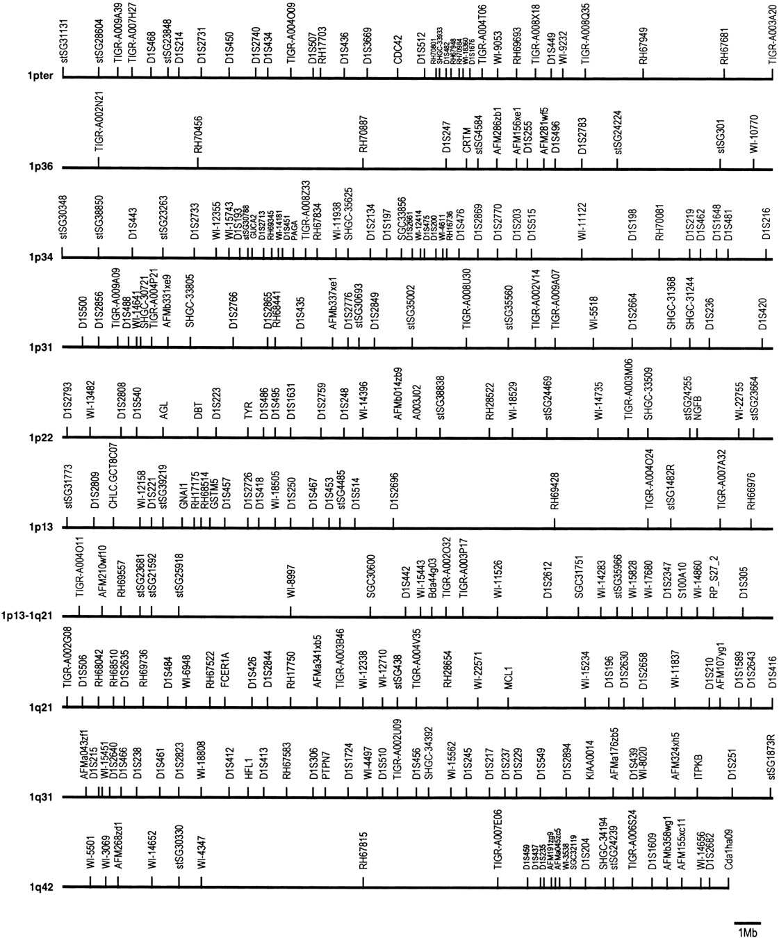
A set of 62 Généthon microsatellite markers that were carefully scored in the GB4 panel served as an initial skeletal map during construction. The skeletal markers were ordered with ≥1000:1 pairwise odds, and the RH- and genetic linkage-determined orders were in complete agreement. Each nonskeletal marker was then analyzed against the skeletal map using MultiMap to determine if it could be added to a unique position on the skeletal map with sufficient statistical support (≥1000:1). The final framework consisted of 289 markers covering the 263 Mb of chromosome 1, yielding an average resolution of 910 kb (Fig. 1). The 1000:1 likelihood intervals of all remaining markers, relative to the framework, were then calculated. A total of 4220 unique markers, representing 5306 sets of primers, were assigned map positions (Table1).
Chromosome 1 RH framework. Framework markers are listed horizontally from top left to bottom right starting at the 1p terminus. Markers are spaced proportionally to their centiRay positions. Cytolocations are indicated at the beginning of each line. An approximate physical scale is represented at bottom right.
Chromosome 1 Mapping Summary
| Map tier | Category | Marker number (% of total)[i] |
| Radiation hybrid | total markers | 5,557 |
| unique markers | 4,442 (80) | |
| mapped markers | 4,220 (76) | |
| skeletal map | 62 (1) | |
| framework map | 289 (7) | |
| resolution, kb | 910 | |
| Genetic linkage | total markers | 820 |
| mapped markers | 788 (96) | |
| skeletal map (from RH frame) | 111 (14) | |
| framework map | 160 (20) | |
| resolution, cM | 2.0 | |
| resolution, Mb | 1.6 | |
| SNP | total SNPs | 239 |
| Transcript | transcribed markers | 3,543 |
| markers in EST clusters | 2,795 (56) | |
| total EST clusters | 1,830 | |
| Physical | unique YACs | 1,930 |
| markers with YACs | 2,275 (45) | |
| unique BACs/PACs | 6,167 | |
| markers with BACs/PACs | 1,199 (24) | |
| Cytogenetic | framework | 110 |
| inferred cytolocations | 4,898 | |
| markers in single bands | 2,686 (54) | |
| Bundles | markers in bundles | 1,796 |
| bundles | 643 | |
| avg. max distance, Mb | 5.2 | |
| avg. min distance, Mb | 1.4 | |
| Totals | mapped markers | 5,008 |
| marker density, kb | 52 | |
| mapped clones | 8,097 | |
| mapped elements | 13,105 |
[i] Percentages calculated against the total number of mapped markers (5008) except for the RH and GL categories, in which the total number of mapped RH or GL markers was used, respectively.
Data Integration
Of the 289 markers on the RH framework, 111 were polymorphic and had been genotyped in the Centre d'Etude du Polymorphisme Humain (CEPH) reference pedigrees (Dausset et al. 1990). In a process analogous to the RH framework construction, these 111 markers were used as a skeletal map to construct a genetic linkage (GL) framework. All chromosome 1-assigned polymorphisms from the CEPHdb v8.1 genotype database were used as the polymorphic marker data set. The resulting GL framework comprised 160 markers ordered with ≥1000:1 odds, yielding resolutions of 2.0 cM and 1.6 Mb (Table 1). An additional 628 polymorphic markers, including commonly used tetranucleotide and intragenic polymorphisms that are often excluded from whole-genome maps, were then placed into 1000:1 likelihood intervals relative to the framework. We also included 239 chromosome 1-specific single nucleotide polymorphisms (SNPs) that had been scored in GB4 (Wang et al. 1998). Overall, the GL and RH tiers totaled 5008 unique marker placements, with an average marker density of 52 kb (Table 1).
Then, we integrated the RH tier, which is largely composed of markers representing transcribed sequences, with the UniGene EST sequence clusters (Boguski and Schuler 1995). Clusters and mapped RH markers sharing an identical EST sequence were associated together. Overall, 3543 of the 4220 RH markers (84%) represented transcripts, and 2795 (79%) of these transcripts were associated with a total of 1830 EST clusters (Table 1).
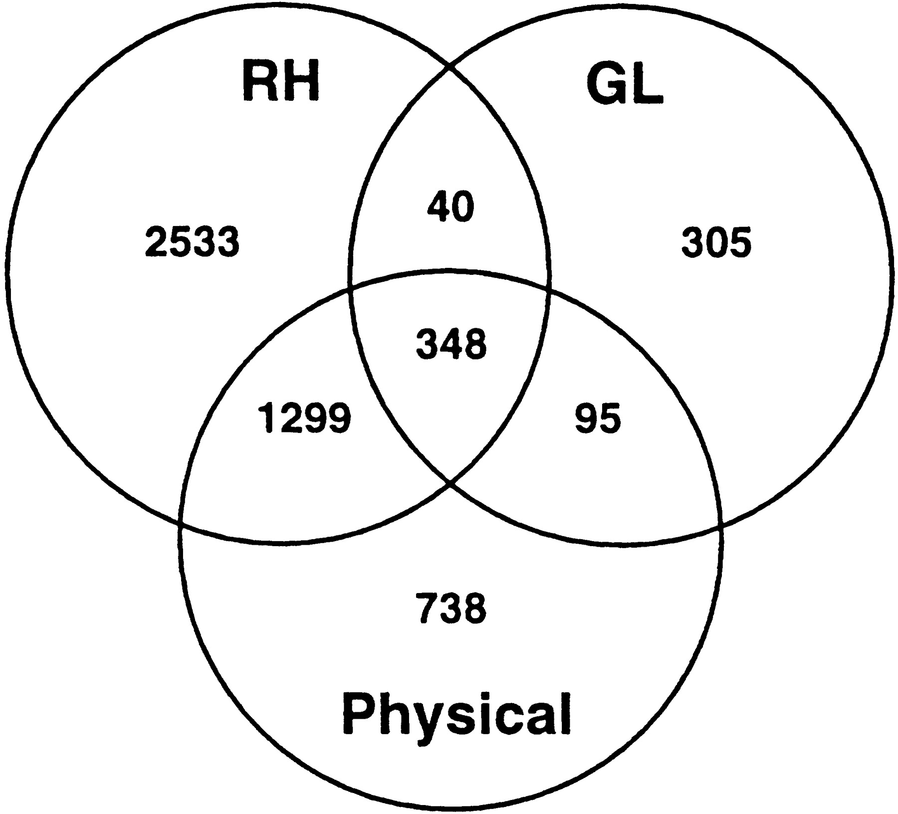
Physical mapping data was integrated by identifying markers for which positive PAC, BAC, or YAC clones have been identified. We determined whether each mapped marker was contained in one or more BAC or PAC clones identified for chromosome 1 sequencing by the Sanger Centre (Gregory et al. 1998), and 6167 BAC/PAC clones representing 1199 chromosome 1 markers were integrated (Table 1). YAC clones containing many of the mapped markers have been isolated by the Whitehead Institute Center for Genome Research (WICGR) (Hudson et al. 1995). A total of 1930 chromosome 1 YACs were added, together representing 2275 markers on the map. The number of markers present and overlapping between the RH, GL, and physical tiers is demonstrated by the Venn diagram in Figure 2.
Venn diagram of marker subtypes. The diagram shows the distribution of markers between and among the RH, GL, and physical tiers. The RH and GL marker sets are defined by all RH and GL markers assigned map positions in CompView (n = 4220 and n = 788), respectively. The physical marker set is defined by the number of unique markers with associated WICGR YACs and/or Sanger PAC/BACs (n = 2480), a subset of which (n = 1742) is localized in CompView.
To include cytogenetic positional information, we used the Genome Database (GDB) (Letovsky et al. 1998) to identify a set of 110 RH tier markers that had been cytogenetically localized to a specific chromosome 1 band. Using these localizations as a cytogenetic framework, inferred cytolocations were then calculated for all remaining GL and RH markers. A single chromosome band could be assigned for 54% (2686) of the cytolocalized markers; the remainder of the markers were assigned a cytogenetic band range.
Representation of larger genomic structures requires a mechanism to identify redundant and partially redundant elements. As RH-based map positions are determined by the amplification of short DNA segments, they can be represented as distinct genomic points. However, functional genomic elements are often more subjectively defined. Thus, a single gene might be represented by multiple markers distributed throughout a large genomic region, with each marker corresponding to a distinct map position. Integration is also complicated by marker nomenclature, such that multiple names are often assigned to the same genomic element. For clarity, we have calculated both the precise localization of each distinct marker and the consensus position of a group of interrelated markers, termed a bundle.
A cumulative list of database identifiers (IDs) was compiled from all markers in Compdb. Markers found to share IDs (essentially sharing an identical name, sequence, or EST cluster) were grouped into bundles that presumably represented transcripts or other functional genomic elements. Each bundle map position was defined from the map positions of the individual markers comprising the bundle. For example, assume bundle X contains three markers with intervaled positions spanning framework markers 1–4, 2–5, and 3–6, respectively. Bundle X would then be represented with a maximum position of 1–6 and a minimum, most likely map position of 3–4. Certain bundles contained markers with nonoverlapping map positions, indicating possible errors in RH scoring, EST cluster building, or identifier labeling. In these cases, bundles were split into subsets of markers with overlapping map positions. Forty-three percent (1796) of the markers could be assembled into 719 bundles, and minimum map positions were defined for 89% of the bundles. For bundles with defined minimum map intervals, the average size of the minimum interval was 1.4 Mb, whereas the average maximum spanned 5.2 Mb. This indicates that the bundling procedure can substantially narrow the most likely location of many transcripts by associating map positions of equivalent markers. The remaining 76 bundles (11%) contained markers with nonoverlapping map positions, and this percentage is largely indicative of the cumulative error rate within the RHdb and UniGene data sets. These nonoverlapping bundles are currently being assessed for the source and reason of the conflicting map positions.
Data Presentation
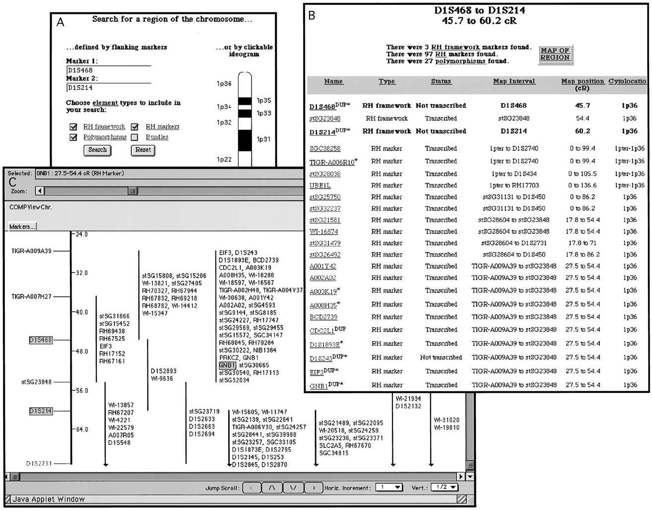
For data presentation, we have developed a CompView internet site (http://genome.chop.edu) that provides graphical and text-based interfaces. The entire chromosome (or subsections that are defined by marker names or cytogenetic bands) can be graphically viewed and customized using the interactive Java applet Mapview (Fig.3) (Letovsky et al. 1998). Information for individual markers includes primer sequences and RH scores, database IDs, EST cluster assignments, inferred cytogenetic positions, and associated large-insert clones (Fig. 4). To supplement the genomic data presented in CompView, hypertext links to external databases are also provided. Currently, direct links to 28 Internet-based databases are included, with specific marker information available for 19 databases (Table 2). These include links to marker or sequence repositories such as dbSTS, dbEST, GenBank, UniGene, RHdb, and GDB; links to individual laboratory or genome center marker databases; real-time queries of large-insert clone screening projects; sequence homology searches using BLAST; and search engine queries using OMIM, BioHunt, and GeneCards (Fig. 4). Thus, the individual marker records presented in CompView serve as a data portal to a wider array of genomic, sequence, and functional data available at other sites.
CompView Web interface examples. (A) Input screen to search for a region of the chromosome. Regions can be defined by two flanking markers (left), by clicking on a cytogenetic band from a chromosome ideogram (right), or by selecting one or a range of cytogenetic bands (not shown). A query input for the region between D1S468 and D1S214 is displayed. (B) Tabular return for the query D1S468 to D1S214 fromA. The marker type, transcriptional status, RH interval, RH map position, and cytolocation are shown for each marker, with a hyperlink to more complete information provided for each marker. Attop is shown the total number of each type of marker found. Clicking on the “map of region” button at top rightyields C. (C) Graphical return of the queryD1S468 to D1S214 viewed with Mapview. In this example, only the RH framework (left) and a portion of the RH markers' tier (right) are visible. CentiRay distances from 1pter are shown at right of the framework. Intervaled RH markers are preceded with a vertical line indicating their 1000:1 likelihood positions relative to the RH framework. The markers used for querying are highlighted on the framework, as is the RH marker forGNB1; clicking on GNB1 yields the marker record shown in Fig. 4.
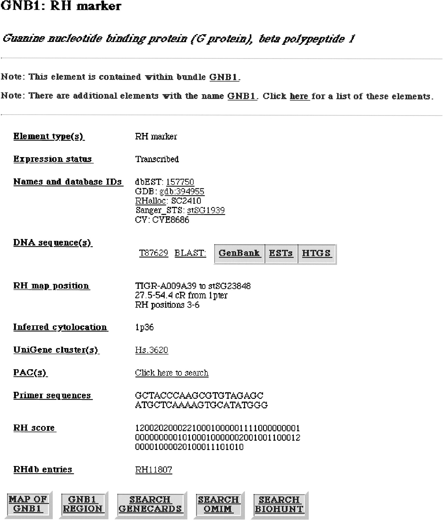
Marker record example. Shown is the individual record for geneGNB1. Underlined text indicates a hypertext link. External database links are present in this example to dbEST (see Table 2 legend for abbreviations), GDB, Sanger, GenBank, UniGene, and RHdb entries for this marker; to perform a BLAST search of the nonredundant (GenBank), EST (EST), and high-throughput genomic sequence (HTGS) collections in GenBank; to search GeneCards, OMIM, and BioHunt for “GNB1”; and to search the Sanger Centre chromosome 1 mapping database Acedb1 for BACs and PACs with the GNB1 primer sequences. The buttons labeled “MAP OF GNB1” and “GNB1 REGION” provide a graphical depiction of the region surrounding GNB1 analogous to Fig. 3 Cand a tabular summary of all markers mapping to this region analogous to Fig. 3 B, respectively. The data category names listed atleft (such as “Expression status”) are hyperlinked to help pages describing the category.
Links to External Databases in the CompView Web Site
[i] Database abbreviations: (ATCC) American Type Culture Collection; (BioHunt) Swiss Institute of Bioinformatics molecular biology internet search engine; (BLAST) Basic Local Alignment Search Tool; (CEPH) Centre d'Etude du Polymorphisme Humain; (CGM-WUSM) Center for Genetics in Medicine, Washington University School of Medicine; (CHLC) Cooperative Human Linkage Center; (dbEST) Expressed Sequence Tag Database; (dbSTS) Sequence-Tagged Site Database; (GDB) Genome Database; (GeneCards) Weizmann Institute human gene catalog; (Genexpress) Généthon EST cataloguing database; (IMAGE) Integrated Molecular Analysis of Genomes and their Expression database; (INSDC) International Nucleotide Sequence Database Collaboration; (KDRI) Kazusa DNA Research Institute; (NHGRI) National Human Genome Research Institute; (OMIM) Online Mendelian Inheritance in Man; (PAGE) Page Laboratory, Whitehead Institute, MIT; (RHalloc) RH EST allocation database; (RHdb) Radiation Hybrid Database; (Salk/GESTEC) University of Texas Southwestern Genome Science and Technology Center; (SC) Sanger Centre; (SHGC) Stanford Human Genome Center; (TIGR) The Institute for Genomic Research; (UCHSC) University of Colorado Health Science Center; (UniGene) UniGene Human Sequences Collection; (UT) University of Utah Genome Center; (WICGR) Whitehead Institute Center for Genome Research; (WTCHG) Wellcome Trust Center for Human Genetics.
[ii] Whether external links point directly to specific data regarding the marker in CompView being viewed.
[iii] Type of search parameter used: (O) oligonucleotide sequences; (S) DNA sequence; (M) marker name or database identifier; (C) DNA clone name.
[iv] Type of data available: (M) genomic mapping; (C) DNA clone; (S) DNA sequence; (E) transcript expression; (F) gene or locus function.
Many markers are associated with multiple names, and sorting through the redundant nomenclature for a given locus is often tedious. To select suitable marker names, we created an algorithm that selects the most appropriate marker name from the pool of database IDs associated with each marker, according to a predetermined name source hierarchy. Bundles were named in a similar manner by selecting from the pool of marker names within each bundle.
Data Integrity
Verification of predicted marker order is a crucial step in map construction. The computational methods used for construction of the RH and linkage tiers were based on standard mapping algorithms that have proven reliable for accurate marker ordering (Matise et al. 1994; Dib et al. 1996; Langston et al. 1999). We also used a number of internal and external comparisons to assess the integrity of our mapping procedure. For internal comparison, we first carefully analyzed the skeletal map to determine whether the RH-defined marker order compared favorably with the order predicted by genetic linkage analysis. Also, for the RH framework, each marker was removed individually and then remapped to confirm localization with sufficient statistical confidence. Moreover, we compared the positions of all markers placed on both the linkage and RH tiers. For all internal comparisons, virtually all marker positions were in agreement. For external verification, we compared our results with those of previously published chromosome 1 maps. The order of our 289 RH framework markers was compared with the corresponding positions on the GeneMap96 RH (Schuler et al. 1996), GeneMap98 RH (Deloukas et al. 1998), and Généthon version 3 GL maps (Dib et al. 1996). The accuracy of the GDB-derived cytogenetic framework was determined by comparison with a set of 212 chromosome 1 large-insert clones that had been cytogenetically mapped by the Sanger Centre in preparation for sequencing. Each comparison showed concordant marker orders for >90% of markers. Almost all discrepancies were found to be isolated, with our predicted marker positions usually adjacent to those in other maps and usually involving markers with weak statistical support for placement. Finally, we compared our marker orders with those predicted by previously published maps of 1p35–36 (Jensen et al. 1997) and 1q41–43 (Weith et al. 1995). Concordancy rates for markers mapped in common were 94% with the distal 1p map and 100% with the distal 1q map. Overall, these comparisons strongly suggest that the CompView method is sound and that isolated variations of marker positions are most likely due to errors in data generation or entry rather than in map construction.
Chromosome 1 Analysis
Several aspects of the chromosome 1 results were analyzed further. Of the 289 RH framework positions, 182 (63%) were definitively assigned to the short arm. This over-representation is likely due to the larger number of 1p-specific RH markers in RHdb, which in turn is due to selective targeting of 1p for STS generation by the Sanger Centre in their chromosome 1 sequencing efforts (Gregory et al. 1998). RH distances are measured in centiRays, which are generally considered proportional to physical distance (Cox et al. 1990). However, inflated RH map distances were observed within the centromeric and adjacent 1q heterochromatic regions (RH framework positionsD1S2696–D1S3356; avg. distance 27.5 cR vs. 12.7 cR for entire framework; P < 0.001), consistent with previous observations for centromeric regions (Benham et al. 1989; Cox et al. 1990; Walter et al. 1994). Several additional regions of low framework marker/centiRay distance were observed, most notably in 1p35 and 1q43 (Fig. 1). These regions may represent local areas of poor marker coverage or increased radioresistance, as both regions overlap dark cytogenetic bands (see below). Although a telomere-specific STS is not yet available for 1p, a recently identified 1q-specific marker (TEL1q-10) (Hudson et al. 1995; Dib et al. 1996) is present in our RH tier, and its map interval includes the 1q telomere. It will be important to anchor future RH maps with telomeric markers as they become available.
Light Giemsa-staining cytogenetic bands are generally considered to be transcript rich (Bernardi 1989). To determine whether this principle holds true for chromosome 1, we calculated the number of transcripts that had been assigned specifically to light and dark bands on our cytogenetic tier. Of 1883 transcripts mapping to a single band, 1663 (88.3%) were assigned to light bands (Table 3). After accounting for the relative size of each band, as previously determined by fractional length measurements (Francke and Oliver 1978), light bands were found on average to be 1.7-fold more likely to contain a transcript than equivalent-sized dark bands, with the light band 1q21 being the most transcript rich. However, there were several notable exceptions to the general trend, including high transcript density for dark band 1p31 and low densities for light bands 1p32, 1p22, 1q23, 1q31, and 1q42.
Cytogenetic Band/Marker Comparison
| Cytogenetic band[i] | Band type | Band size[ii] | Number of transcripts | Transcript density[iii] |
| 1p36 | light | 0.12 | 447 | 1.24 |
| 1p34 | light | 0.025 | 185 | 2.46 |
| 1p32 | light | 0.085 | 7 | 0.03 |
| 1p31 | dark | 0.045 | 173 | 1.28 |
| 1p22 | light | 0.06 | 123 | 0.68 |
| 1p21 | dark | 0.03 | 41 | 0.45 |
| 1p13 | light | 0.025 | 206 | 2.74 |
| 1q21 | light | 0.025 | 287 | 3.81 |
| 1q23 | light | 0.095 | 19 | 0.07 |
| 1q31 | dark | 0.04 | 6 | 0.05 |
| 1q32 | light | 0.045 | 386 | 2.85 |
| 1q42 | light | 0.03 | 3 | 0.03 |
| Total, chromosome | 0.625 | 1883 | 1.00 | |
| Total, light bands | 0.51 | 1663 | 1.08 | |
| Total, dark bands | 0.115 | 220 | 0.63 | |
| Ratio, light:dark | 1.70 |
[i] Only bands for which one or more framework cytogenetic markers had been uniquely assigned to are included in the analysis.
[ii] Fractional length of chromosome 1 for each band.
[iii] Relative transcript density, calculated as a ratio relative to the total chromosome density; calculation specifics detailed in Methods.
DISCUSSION
We have established a method of constructing comprehensive representations of chromosomes that gives a multifaceted view of a given genome. CompView has several advantages over most current methods for map construction. First, we have been able to relate mapping data from publicly available sources that are derived from differing experimental approaches, including cytogenetic, genetic linkage, and physical localization methods. Second, the dynamic framework approach creates maps with very high resolution that also retain high statistical support for marker order. For example, our chromosome 1 RH framework consists of 289 markers ordered with ≥1000:1 likelihood odds, which establishes two- to three-fold higher resolution than existing genome maps (Hudson et al. 1995; Stewart et al. 1997;Deloukas et al. 1998; Gregory et al. 1998). Third, the process of marker integration allows greater numbers of markers and large-insert clones (>13,000 combined) to be positioned than do existing maps, which mainly rely on a single experimental technique. The subsequent increase in marker and clone density strengthens the utility of the map for downstream applications. Fourth, we have fully integrated cytogenetic localization data, a critical requirement for genetic disease searches that are often driven by karyotype-based clinical observations, but an aspect lacking in other recent maps. Finally, the EST bundling procedure uses positional, descriptive, and functional information to determine the integrity of EST clustering algorithms, to define more precise localizations, and to more effectively manage marker and gene nomenclature.
The initiation of the chromosome 1 CompView project was largely motivated by the lack of coherence in currently available genomic information. The large number of groups, methodologies, nomenclature schemes, and data sets makes data mining of specific loci difficult, especially for new investigators unfamiliar with the wide range of genomic resources available. The CompView Web site accommodates researchers who define loci by differing parameters, such as clinical (e.g., a cytogenetic band) and genetic (e.g., a polymorphism) means. Users are then provided with precise information regarding an individual locus or a summary of the region of interest. This information in turn leads to additional data through the external links provided. In this way, CompView provides both a convenient genome-based summary of the interesting locus or region and a marker-specific portal to additional information. CompView can be easily used to view other human chromosomes, and with some modifications can be adapted for integration of proprietary data sources or analysis of other complex genomes.
The HGP is well underway in establishing the complete DNA sequence of the human genome, and mapping efforts in several other mammalian organisms are progressing rapidly (Rohrer et al. 1996; Kappes et al. 1997; McCarthy et al. 1997; Mellersh et al. 1997; Brown et al. 1998; de Gortari et al. 1998). Although a rough draft of the human genome sequence is imminent, most genetic disease-oriented research proceeds from chromosomal or regional localization to specific DNA sequence rather than the reverse. Thus, the development of more sophisticated bioinformatics tools to streamline the transition from genomic position to DNA sequence will be important both for large-scale genomic analyses and for individual locus characterizations (Collins et al. 1998). Besides attaining increased map resolution, CompView creates such a transition by serving as a portal between specific genomic landmarks and relevant genomic and functional data. Furthermore, chromosome views can serve both as physical and organizational scaffolds and for regional, chromosomal, and organism-wide sequencing projects, whereas the localized placement of large-insert clones is useful for the assembly of sequence-ready contigs. For example, retrieving a list of CompView markers and corresponding map positions that do not have associated PAC or BAC clones could be used to quickly determine which regions of a chromosome require additional clone coverage for mapping and/or sequencing. As the RH-based nature of CompView reflects approximate physical distance, marker density and clone coverage within specific regions can be assessed and used to determine where additional efforts are required.
Currently, linkage-based searches for complex genetic loci usually identify large regions, so improved precision, accuracy, and density of genome maps can greatly reduce positional candidate gene searches. As an example, CompView has been used to identify and determine the potential tumor suppressor candidacy of transcripts within a region of allelic loss on 1p36 defined in neuroblastomas (White et al. 1999). Likewise, improved maps augment the capacity of high-throughput genomic screening and functional genomic technologies, including DNA microarraying (Chee et al. 1996), SNP analysis (Wang et al. 1998), genome mismatch scanning (Cheung et al. 1998), and novel genetic linkage algorithms for identifying complex disease traits (Darvasi 1998). Moreover, the complete integration of structural genomic information is an important prerequisite toward functional-based descriptions of whole cells, which would incorporate information derived from functional genomic and proteomic-based experimental approaches (Fields 1997; Strachan et al. 1997). Fully computation-based representations of entire genomes may soon be possible by merging positional, observational, and functional data in a manner similar to the CompView procedure.
METHODS
Comprehensive View Database and Web Site
Compdb is a relational database that was written in the 4th Dimension (4D) language (ACI, Cupertino, CA). Procedures for data parsing and analysis were also written in 4D and incorporated into the Compdb database structure. A custom-designed graphical user interface was built for Compdb, which allows convenient viewing and reporting of imported data. The CompView Web site is served by WebSTAR (StarNine Technologies, Berkeley, CA), and queries are linked to Compdb through NetLink/4D (Foresight Technology, Fort Worth, TX) using the Common Gateway Interface standard. Data for graphical queries are translated into the CTL language and returned to the Mapview Java applet loaded on the client machine, whereupon Mapview converts the CTL file into a graphical image.
RH and GL Tier Construction
RH marker data from RHdb version 11 was parsed into Compdb. Entries with identical primer pair sequences were related to a common marker record. Scoring data and/or marker information from skeletal RH and all GL markers were parsed into Compdb in a manner similar to the RH data parsing. Where possible, these entries were related to existing markers. Skeletal marker RH scores were used preferentially for their related markers. Scoring data from all marker records assigned to chromosome 1 and scored in the GB4 panel were exported to MultiMap.
Unique chromosome 1 GB4 markers were initially tested for linkage to each other, with an odds threshold for linkage grouping set at ≥1000:1. Markers not sufficiently linked to at least one member of the main linkage group (n = 21) were removed. A set of 62 well-ordered Généthon microsatellite markers, derived from the wEST framework maps (www.well.ox.ac.uk/∼james/GB4), was used as an initial skeletal map (see Note 23 in Schuler et al. 1996). Markers were then analyzed against the skeletal map using MultiMap to determine if they could be added to a unique position on the skeletal map with sufficient statistical support. The framework was first constructed by adding markers with an odds threshold ≥10,000:1 and then with odds ≥1000:1 in an iterative process, preferentially adding polymorphic markers. Each marker on the resulting framework was then individually removed from the framework and remapped. Markers not localized to the same unique position with ≥1000:1 odds were removed from the framework. The 1000:1 likelihood intervals of all remaining RH markers relative to the framework were then calculated. Markers whose intervals measured >10% of the entire framework length were removed (n = 201).
A GL skeletal map was established by using the subset of RH framework markers that were also polymorphic. Only the subset of markers whose GL order was consistent with the RH order were included in the skeletal map. Analogous to the RH framework construction, the GL skeletal map was then used as a basis for dynamically building a GL framework, again by iteratively invoking MultiMap. Subsequently, 1000:1 likelihood intervals for the remaining polymorphic markers previously assigned to chromosome 1 were placed relative to the framework. Following MultiMap analysis, map positions for all GL- and RH-based markers were parsed into Compdb.
Naming of Markers and Bundles
Markers were assigned appropriate names from the set of all IDs belonging to the RHdb or CEPHdb records related to each marker. Markers were named by HUGO nomenclature committee-approved gene symbol (White et al. 1997) if available, followed by D-number. If neither was available, names were selected by Genome Center-assigned IDs, with the Genome Centers ranked by the number of RH entries submitted to RHdb, then by sequence accession number, dbEST ID, dbSTS ID, and RHalloc db ID, in the order listed. Bundles were named from the pool of component marker names in an analogous manner.
EST Cluster Integration and Bundle Construction
Build 88 (August 4, 1999) of UniGene was used for the statistics presented here. DNA sequence IDs for each marker were used to query UniGene and identify corresponding EST clusters, which were then related to the marker records. Markers were then grouped into bundles if they shared a common database identifier, including DNA sequence, dbEST, dbSTS, or UniGene cluster IDs. After analysis of the marker map positions comprising each bundle, the bundles were divided into three groups depending on whether the component marker positions all shared a common map position or interval (overlapping), together defined a contiguous map interval but where a common interval shared by all marker positions could not be defined (continuous), or defined two or more noncontiguous map intervals (split). Maximum (max) and minimum (min) bundle map positions were calculated for overlapping bundles, using the marker map positions closest to the 1p and 1q termini as the max and the positions defining the shared overlapping region as the min. Only max positions were calculated for continuous bundles. Split bundles were separated into the minimum set of subbundles or individual markers that could be defined as either overlapping or continuous.
Integration with Cytogenetic and Physical Data
For cytogenetic integration, primer pair sequences for all mapped markers were used to search GDB to identify corresponding cytolocations. Markers with cytolocations restricted to a single band or less were used as a cytogenetic framework, with sub-bands being rounded to their parent bands (e.g., 1p36.3 to 1p36). The cytogenetic framework was manually checked for consistency, and outlying markers were removed from the framework if substantial, conflicting localizations were available. All RH framework positions were assigned a cytogenetic band or range according to the RH map positions or ranges of each marker on the cytogenetic framework. All other markers were then given inferred cytolocations by converting marker RH map intervals to the cytogenetic bands assigned to all RH framework positions comprising the interval.
YAC data from WICGR release 12 were parsed into Compdb. Only unambiguous YAC addresses that had been identified with primer sequences identical to those of markers in Compdb were added. WICGR SNP markers, from WICGR SNP release 1, are a subset of existing RHdb entries and were annotated as such by matching SNP primer sequences with RH marker primer sequences. BAC and PAC integration was achieved via the Web site interface, where a hypertext link is provided from each marker page that invokes a query of the Sanger Centre chromosome 1 database (1ace) to search for BACs/PACs identified with the marker primers.
Cytogenetic Band/Transcript Analysis
Calculations of transcript numbers in light and dark cytogenetic bands were performed using the subset of markers known to be transcribed and that had been assigned to a single band. Comparison by band size used fractional length measurements from Francke and Oliver (1978). Transcript densities for each band, as listed in Table 3, were calculated as the number of transcripts mapping specifically to the band, divided by the product of the fractional length of the band and the total number of transcripts for the whole chromosome. The light/dark transcript ratio was calculated as the sum of all transcript densities for each light band divided by the sum of all transcript densities for each dark band.
We gratefully acknowledge the Human Genome Centers and public databases for access to unpublished genomic data; M. James for the skeletal marker RH scores; A. Chakravarti, C. Kashuk, J. Ott, and M. Boehnke for helpful discussions; P. Rodriguez-Tomé for help with RHdb data; L. Kramer for Mapview assistance; S. Gregory and C. Scott for analysis of Sanger Centre data; K. Richardson for graphical assistance; and R. Spielman, G. Brodeur, M. Hogarty, J. Maris, and J. Biegel for advice during preparation of this manuscript. This work was supported in part by a Joseph Stokes Jr. Research Institute High Risk/High Impact Grant (to P.S.W.) and by National Institutes of Health grants HG01691 and HG00008 (to T.C.M.).
The publication costs of this article were defrayed in part by payment of page charges. This article must therefore be hereby marked “advertisement” in accordance with 18 USC section 1734 solely to indicate this fact.
Notes
[9] Corresponding author.
Notes
[10] E-MAIL [email protected]; FAX (215) 590-3770.
REFERENCES
- ↵F. BenhamK. HartJ. CrollaM. BobrowM. FrancavillaP.N. Goodfellow(1989) A method for generating hybrids containing nonselected fragments of human chromosomes. Genomics 4:509–517.
- ↵G. Bernardi(1989) The isochore organization of the human genome. Annu. Rev. Genet. 23:637–661.
- ↵M.S. BoguskiG.D. Schuler(1995) ESTablishing a human transcript map. Nat. Genet. 10:369–371.
- ↵D.M. BrownT.C. MatiseG. KoikeJ.S. SimonE.S. WinerS. ZangenM.G. McLaughlinM. ShiozawaO.S. AtkinsonJ.R.J. Hudson(1998) An integrated genetic linkage map of the laboratory rat. Mamm. Genome 9:521–530.
- ↵M. CheeR. YangE. HubbellA. BernoX.C. HuangD. SternJ. WinklerD.J. LockhartM.S. MorrisS.P.A. Fodor(1996) Accessing genetic information with high-density arrays. Science 274:610–614.
- ↵V.G. CheungJ.P. GreggK.J. Gogolin-EwensJ. BandongC.A. StanleyL. BakerM.J. HigginsN.J. NowakT.B. ShowsW.J. Ewens(1998) Linkage-disequilibrium mapping without genotyping. Nat. Genet. 18:225–230.
- ↵F.S. Collins(1995) Positional cloning moves from perditional to traditional. Nat. Genet. 9:347–350.
- ↵F.S. CollinsA. PatrinosE. JordanA. ChakravartiR. GestelandL. Walters(1998) New goals for the U.S. Human Genome Project: 1998–2003. Science 282:682–689.
- ↵D.R. CoxM. BurmeisterE.R. PriceS. KimR.M. Myers(1990) Radiation hybrid mapping: A somatic cell genetic method for constructing high-resolution maps of mammalian chromosomes. Science 250:245–250.
- ↵A. Darvasi(1998) Experimental strategies for the genetic dissection of complex traits in animal models. Nat. Genet. 18:19–24.
- ↵J. DaussetH. CannD. CohenM. LathropJ.M. LalouelR. White(1990) Centre d'Etude du Polymorphisme Humain (CEPH): Collaborative genetic mapping of the human genome. Genomics 6:575–577.
- ↵M.J. de GortariB.A. FrekingR.P. CuthbertsonS.M. KappesJ.W. KeeleR.T. StoneK.A. LeymasterK.G. DoddsA.M. CrawfordC.W. Beattie(1998) A second-generation linkage map of the sheep genome. Mamm. Genome 9:204–209.
- ↵P. DeloukasG.D. SchulerG. GyapayE.M. BeasleyC. SoderlundP. Rodriguez-ToméL. HuiT.C. MatiseK.B. McKusickJ.S. Beckmann(1998) A physical map of 30,000 human genes. Science 282:744–746.
- ↵C. DibS. FauréC. FizamesD. SamsonN. DrouotA. VignalP. MillasseauS. MarcJ. HazanE. Seboun(1996) A comprehensive genetic map of the human genome based on 5,264 microsatellites. Nature 380:152–154.
- ↵S. Fields(1997) The future is function. Nat. Genet. 15:325–327.
- ↵U. FranckeN. Oliver(1978) Quantitative analysis of high-resolution trypsin-Giemsa bands on human prometaphase chromosomes. Hum. Genet. 45:137–165.
- ↵S.G. GregoryM. VaudinR. WoosterD. MischkeM. ColemanC. PorterB.C. SchutteP. WhiteJ.M. Vance(1998) Report of the Fourth International Workshop on Human Chromosome 1 Mapping. Cytogenet. Cell Genet. 78:154–182.
- ↵G. GyapayK. SchmittC. FizamesH. JonesN. Vega-CzarnyD. SpilletD. MuseletJ.F. Prud'HommeC. DibC. Auffray(1996) A radiation hybrid map of the human genome. Hum. Mol. Genet. 5:339–346.
- ↵T.J. HudsonL.D. SteinS.S. GeretyJ. MaA.B. CastleJ. SilvaD.K. SlonimR. BaptistaL. KruglyakS.-H. Xu(1995) An STS-based map of the human genome. Science 270:1945–1954.
- ↵S.J. JensenE.P. SulmanJ.M. MarisT.C. MatiseP.J. VojtaJ.C. BarrettG.M. BrodeurP.S. White(1997) An integrated transcript map of human chromosome 1p35-p36. Genomics 42:126–136.
- ↵S.M. KappesJ.W. KeeleR.T. StoneR.A. McGrawT.S. SonstegardT.P. SmithN.L. Lopez-CorralesC.W. Beattie(1997) A second-generation linkage map of the bovine genome. Genome Res. 7:235–249.
- ↵A.A. LangstonC.S. MellershN.A. WiegandG.M. AclandK. RayG.D. AguirreE.A. Ostrander(1999) Toward a framework linkage map of the canine genome. J. Hered. 90:7–14.
- ↵S.I. LetovskyR.W. CottinghamC.J. PorterP.W.D. Li(1998) GDB: The Human Genome Database. Nucleic Acids Res. 26:94–99.
- ↵P. LijnzaadC. HelgesenP. Rodriguez-Tomé(1998) The Radiation Hybrid Database. Nucleic Acids Res. 26:102–105.
- ↵T.C. MatiseM. PerlinA. Chakravarti(1994) Automated construction of genetic linkage maps using an expert system (MultiMap): A human genome linkage map. Nat. Genet. 6:384–390.
- ↵L.C. McCarthyJ. TerrettM.E. DavisC.J. KnightsA.L. SmithR. CritcherK. SchmittJ. HudsonN.K. SpurrP.N. Goodfellow(1997) A first-generation whole genome–radiation hybrid map spanning the mouse genome. Genome Res. 7:1153–1161.
- ↵C.S. MellershA.A. LangstonG.M. AclandM.A. FlemingK. RayN.A. WiegandL.V. FranciscoM. GibbsG.D. AguirreE.A. Ostrander(1997) A linkage map of the canine genome. Genomics 46:326–336.
- ↵N. RischK. Merikangas(1996) The future of genetic studies of complex human diseases. Science 273:1516–1517.
- ↵G.A. RohrerL.J. AlexanderZ. HuT.P. SmithJ.W. KeeleC.W. Beattie(1996) A comprehensive map of the porcine genome. Genome Res. 6:371–391.
- ↵The Sanger Centre and The Washington University Genome Sequencing Center (1998) Toward a complete human genome sequence. Genome Res. 8:1097–1108.
- ↵G.D. SchulerM.S. BoguskiE.A. StewartL.D. SteinG. GyapayK. RiceR.E. WhiteP. Rodriguez-ToméA. AggarwalE. Bajorek(1996) A gene map of the human genome. Science 274:540–546.
- ↵E.A. StewartK.B. McKusickA. AggarwalE. BajorekS. BradyA. ChuN. FangD. HadleyM. HarrisS. Hussain(1997) An STS-based radiation hybrid map of the human genome. Genome Res. 7:422–433.
- ↵T. StrachanM. AbitbolD. DavidsonJ.S. Beckmann(1997) A new dimension for the human genome project: Towards comprehensive expression maps. Nat. Genet. 16:126–132.
- ↵M.A. WalterD.J. SpillettP. ThomasJ. WeissenbachP.N. Goodfellow(1994) A method for constructing radiation hybrid maps of whole genomes. Nat. Genet. 7:22–28.
- ↵D.G. WangJ.-B. FanC.-J. SiaoA. BernoP. YoungR. SapolskyG. GhandourN. PerkinsE. WinchesterJ. Spencer(1998) Large-scale identification, mapping, and genotyping of single-nucleotide polymorphisms in the human genome. Science 280:1077–1082.
- ↵A. WeithG.M. BrodeurG.A.P. BrunsT.C. MatiseD. MischkeD. NizeticM.F. SeldinN. Van RoyJ. Vance(1995) Report of the second International Workshop on Human Chromosome 1 Mapping 1995. Cytogenet. Cell Genet. 72:114–144.
- ↵J.A. WhiteP.J. McAlpineS. AntonarakisH. CannJ. EppigK. FrazerJ. FrezalD. LancetJ. NahmiasP. Pearson(1997) Guidelines for human gene nomenclature. Genomics 45:468–471.
- ↵White, P.S., P.M. Thompson, B.A. Seifried, E.P. Sulman, S.J. Jensen, C. Guo, J.M. Maris, M.D. Hogarty, C. Allen, J.A. Biegel et al. 1999. Detailed molecular analysis of 1p36 in neuroblastoma. Eur. J. Cancer (in press)..