
STCC enhances spatial domain detection through consensus clustering of spatial transcriptomics data
- 1Center for Single-Cell Omics, School of Public Health, Shanghai Jiao Tong University School of Medicine, Shanghai 200025, China;
- 2Key Laboratory of Carcinogenesis and Translational Research (Ministry of Education/Beijing), Department of Lymphoma, Peking University Cancer Hospital and Institute, Beijing 100142, China;
- 3The Guangxi Key Laboratory of Intelligent Precision Medicine, Guangxi Zhuang Autonomous Region, Nanning 530007, China;
- 4Center for Precision Medicine Multi-Omics Research, Institute of Advanced Clinical Medicine, Peking University, Beijing 100191, China;
- 5Department of Biomedical Informatics, School of Basic Medical Sciences, Peking University Health Science Center, Beijing 100191, China
Abstract
The rapid advance of spatially resolved transcriptomics technologies has yielded substantial spatial transcriptomics data. Deriving biological insights from these data poses nontrivial computational and analysis challenges, of which the most fundamental step is spatial domain detection (or spatial clustering). Although a number of tools for spatial domain detection have been proposed in recent years, their performance varies across data sets and experimental platforms. It is thus an important task to take full advantage of different tools to get a more accurate and stable result through consensus strategy. In this work, we developed STCC, a novel consensus clustering framework for spatial transcriptomics data that aggregates outcomes from state-of-the-art tools using a variety of consensus strategies, including Onehot-based, average-based, hypergraph-based, and wNMF-based methods. Comprehensive assessments on simulated and real data from distinct experimental platforms show that consensus clustering significantly improves clustering accuracy over individual methods under varied input parameters. For normal tissue samples exhibiting clear layered structure, consensus clustering by integrating multiple baseline methods leads to improved results. Conversely, when analyzing tumor samples that display scattered cell type distribution patterns, integration of a single baseline method yields satisfactory performance. For consensus strategies, average-based and hypergraph-based approaches demonstrate optimal precision and stability. Overall, STCC provides a scalable and practical solution for spatial domain detection in spatial transcriptomics data, laying a solid foundation for future research and applications in spatial transcriptomics.
Spatially resolved transcriptomics (SRT) techniques, which quantify gene expression profiles while preserving cellular spatial information, have emerged as a key technology for interrogating cell heterogeneity and tissue development (Bäckdahl et al. 2021). Leveraging SRT, researchers have delineated spatiotemporal transcriptomic landscapes across various developmental stages of human and mouse tissues such as brain and embryo (Sato et al. 2008; Moffitt et al. 2018; Carlberg et al. 2019; Chen et al. 2022; Zhang et al. 2023), offering useful insights into mammalian tissue development. Meanwhile, SRT has also been instrumental in elucidating mechanisms underlying complex disorders such as cancer (Berglund et al. 2018; Vickovic et al. 2019; Ji et al. 2020), rheumatoid arthritis (Vickovic et al. 2022), diabetes (Theocharidis et al. 2022), and Parkinson's (Jia et al. 2023) and Alzheimer's diseases (Chen et al. 2020) by probing disease-associated alterations in spatial gene expression patterns. Such investigations can potentially inform early biomarkers and therapeutic targets for complex diseases (Brennecke et al. 2013).
Depending on the platform adopted, SRT technologies quantify gene expression across scales of multicellular, single-cell, and subcellular resolutions (Dries et al. 2021), with representative technologies of 10x Genomics Visium, STARmap (Wang et al. 2018), and Stereo-seq (Chen et al. 2022), respectively. These multiresolution SRT data sets empower diverse downstream analyses including spatial domain detection (Liu et al. 2022; Yang et al. 2022; Chidester et al. 2023; Xu et al. 2024a), deconvolution (Andersson et al. 2020; Dong and Yuan 2021; Elosua-Bayes et al. 2021; Song and Su 2021), inference of spatially variable genes (SVGs) (Lopez et al. 2019; Welch et al. 2019; Abdelaal et al. 2020; Biancalani et al. 2021), cell–cell communication (Peng et al. 2022; Shao et al. 2022; Cang et al. 2023; Li et al. 2023; Raredon et al. 2023), and trajectory inference (Zhang et al. 2021; Shen et al. 2025). Among them, spatial domain detection is a crucial and pivotal step for many downstream tasks. For example, the cell type annotation of spatial domains is a prerequisite for understanding their interactions or communications within the tissue, as well as identification of spatial biomarkers across tissue. Recently, a number of algorithms including statistical (e.g., BASS [Li and Zhou 2022], BayesSpace [Zhao et al. 2021], SpatialPCA [Shang and Zhou 2022]) and deep learning (e.g., SEDR [Xu et al. 2024a], stLearn [Pham et al. 2023], SpaGCN [Hu et al. 2021], and STAGATE [Dong and Zhang 2022]) algorithms have been developed for spatial domain detection. However, their performances remain inconsistent across data sets and parameter settings (Cui et al. 2021; Hu et al. 2024; Yuan et al. 2024), making the selection of tools, parameters, and integration of multiple clustering outcomes a challenging task.
One possible strategy to overcome the above challenge is consensus clustering, which aims to integrate multiple methods for enhanced accuracy and robustness (Hore et al. 2009). Consensus clustering has been widely adopted in bulk and scRNA-seq data (e.g., SC3 [Kiselev et al. 2017] and SAFE-clustering [Yang et al. 2019]). Basically, these methods apply diverse dimensionality reduction or resampling techniques on the gene expression matrix, followed by the same or different clustering algorithms to get a series of clustering outputs. Then, individual clustering results are integrated, through consensus matrices or hypergraph segmentation algorithms, to determine consensus clustering labels. Such consensus approaches have demonstrated significant potential to improve the clustering accuracy and stability of bulk and scRNA-seq transcriptomics data (Gan et al. 2018; Cui et al. 2021). However, to the best of our knowledge, consensus clustering frameworks crafted for spatial transcriptomics (ST) data remain scarce. Systematic assessments of clustering accuracy and robustness across various consensus frameworks are lacking.
To address this gap, we here encapsulated and implemented four consensus clustering frameworks, namely, Onehot-based, average-based, hypergraph-based, and weighted nonnegative matrix factorization (wNMF)-based methods, using clustering outcomes of seven typical spatial clustering algorithms as input. To systematically evaluate the performances of these four consensus strategies in terms of ST clustering accuracy and stability, we conducted comprehensive simulations and real data applications across different tissue origins and sequencing platforms. The findings of this comprehensive analysis yield a rich source of references and insights, aimed to guide and enhance future consensus clustering endeavors in ST.
Results
STCC overview
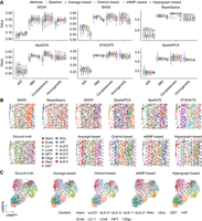
In this work, we present spatial transcriptome consensus clustering (STCC), a consensus framework tailored for clustering of ST data (Fig. 1A). STCC amalgamates multiple clustering results from baseline algorithms through construction of a hypergraph matrix or a consensus matrix. It currently implements four consensus strategies, namely, Onehot-based, average-based, hypergraph-based, and wNMF-based to get final consensus output (for detail, see Methods). Among them, Onehot- and average-based strategies derive consensus labels by simply applying k-means clustering to the corresponding hypergraph matrix or consensus matrix; hence, they are referred to as naive consensus strategies. Two other approaches, namely, hypergraph-based and wNMF-based strategies, obtain consensus labels by employing more advanced algorithms, including hypergraph partitioning, nonnegative matrix factorization, and quadratic programming; they are termed advanced strategies. The efficacy of these consensus strategies is validated using diverse clustering evaluation metrics (for detail, see Methods).
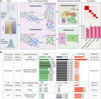
STCC architecture and evaluation data sets. (A) STCC architecture. STCC takes clustering results of seven baseline algorithms as input. It first constructs a hypergraph matrix and a consensus matrix and then executes two naive strategies (average-based, Onehot-based) and two advanced strategies (hypergraph-based, wNMF-based) to get consensus results. The ultimate clustering results are evaluated using seven benchmark metrics, namely, ARI, NMI, completeness score, homogeneity score, Calinski–Harabasz score, Davies–Bouldin score, and stability. (B) Details of seven benchmark data sets, including sequencing technologies, species, organism/disease types, numbers of spots, genes, and cell types, etc.
To comprehensively assess the performance of these diverse consensus strategies, we have collected seven SRT data sets with manual annotations by pathologists as ground truth. These data sets are obtained from various sequencing platforms, species, and tissue origins (Fig. 1B); thus, they hold great diversity for evaluation of a consensus strategy. Subsequently, we applied seven spatial domain detection algorithms as baseline clustering methods to each data set (Supplemental Fig. S1A) and generated 10 distinct outcomes per algorithm by varying parameters or random seeds. Finally, we systematically evaluated the impact of different clustering inputs on the performance of consensus frameworks and specifically compared two scenarios: incorporating multiple clustering results from the same baseline clustering algorithm as input (termed as “single method”), and integrating results from all seven baseline algorithms as input (termed as “all methods”).
STCC enhances clustering performance on simulated data sets
We first evaluated the performance of consensus strategies using simulated data (Fig. 2). To achieve it, we generated a series of simulation data sets on the basis of mouse embryo data by Stereo-seq and mouse brain data by 10x Visium to investigate the influence of different factors, including numbers of spots, highly/spatially variable genes, levels of noise, and cell type numbers (for detail, see Methods). Taking SpaGCN as the baseline algorithm, we observed that when the proportions of highly variable genes (HVGs) and SVGs increase, clustering accuracy of baseline algorithm increases (from 0.5 to 0.62 for HVGs and 0.37 to 0.63 for SVGs) and reaches saturation at around 1800 HVGs and 2400 SVGs. Similar patterns are observed for all consensus strategies, highlighting the important role of HVGs and SVGs on clustering performance irrespective of single or consensus strategies usage (Fig. 2A,B). Increasing noise ratio corresponds to decreasing ARI, but consensus strategies are more tolerant across noise ratios (Fig. 2C; Supplemental Fig. S1C). For example, ARIs for average-based and Onehot-based consensus strategies decrease from 0.69 to 0.18 upon adding noise but still exceed baseline performance (Fig. 2C). We observed fluctuating but overall stable ARI as the number of cell types increased, when consensus strategies show consistently higher performance than the baseline algorithm (Fig. 2D; Supplemental Fig. S1D).
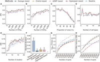
STCC performance on simulated data sets. (A,B) Line plots displaying the ARI for spatial domain detection on simulated data sets across different consensus strategies and baseline methods, with the y-axis showing how ARI varies as the number of added HVGs (A) and SVGs (B) increases. (ARI) Adjusted Rand index, (HVGs) highly variable genes, (SVGs) spatially variable genes. (C,D) Line plots showing the ARI by different consensus strategies and baseline method for spatial domain detection across simulated data sets change (y-axis) with the addition proportions of noise ratio (C) and number of cell types (D). (E) Line plot showing the ARI variation with the number of clusters. (F) The bar plots displaying the standard deviation of ARI from E for both the baseline algorithms and the four consensus strategies. (G,H) The runtimes (G) and maximum memory usage (H) of consensus strategies with varying spot numbers.
We next evaluated the impact of input cluster numbers on the performance of different consensus strategies. By fixing the true cluster number at 15 in simulation data, we varied the input cluster number k from five to 20 (Fig. 2E). The results indicate that consensus clustering methods exhibited greater robustness compared with the baseline clustering method (SpaGCN) when the input cluster number deviated from the true number. Specifically, for consensus strategies, clustering accuracy remained above 0.5 for k-values from nine to 20, peaking at k = 18, which closely aligns with the true cluster number (Fig. 2E). Additionally, we calculated the standard deviation of the ARI for the baseline algorithms and four consensus strategies across different k-values. Compared to the baseline algorithms, the consensus strategies exhibited significantly lower standard deviations than the baseline, indicating more consistent clustering performance (Fig. 2F). Overall, consensus strategies enhanced clustering accuracy and noise resistance to a certain extent compared with the baseline clustering algorithm.
We then compared the runtime and memory usage of consensus strategies as well as baseline method. For runtime, the wNMF-based consensus strategy takes five to 10 times longer runtimes than naive strategies as the number of spots increased (Fig. 2G), which is anticipated owing to its iterative computation procedure. Regarding memory usage, the patterns are slightly different. Average-based, Onehot-based, and wNMF-based strategies generally require more memory than baseline methods (Fig. 2H), primarily owing to the necessity of constructing a N × N connectivity matrix. In contrast, the hypergraph-based consensus strategy shows markedly lower memory consumption.
Consensus clustering achieves enhanced performance over individual baseline algorithms
We next assessed the impact of four consensus strategies on real SRT data using clustering results of single baseline algorithms as input. To this aim, we applied consensus strategies to seven baseline algorithms on mouse brain data and evaluated their performance via seven metrics, namely, ARI, NMI, completeness score, homogeneity score, Calinski–Harabasz score, Davies–Bouldin score, and stability (Fig. 3A; Supplemental Fig. S3A). We found that, in most cases, clustering outcomes show moderate enhancements after applying different types of consensus strategies. More importantly, compared to the baseline algorithms, consensus strategies show reduced variance in all evaluation metrics, especially notable in the “SEDR only” and “SpatialPCA only” scenarios (Fig. 3A). A direct comparison of ARI scores (Fig. 3B) shows consensus strategies consistently outperform baseline algorithms, as evidenced by data points predominantly lying above the diagonal line. In Figure 3C, we visualized the outcomes of consensus clustering using BASS as baseline algorithm. Specifically, all four consensus strategies successfully reconstructed the Cortex_2 region, whereas the baseline algorithm incorrectly identifies it as striatum. Of note, the wNMF-based strategy even exclusively reconstructed the Cortex_5 structure, aligning well with the ground truth (Fig. 3C).
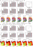
Performance of consensus strategies on single clustering algorithms. (A,D) Consensus clustering accuracies based on single baseline algorithms for the mouse brain data (A) and the DLPFC sample 151675 (D). Each baseline algorithm and consensus strategy are repeated 10 times to calculate the error bars. (B,E) Scatter plot comparing the ARI between baseline methods (x-axis) and consensus strategies (y-axis) for mouse brain data (B) and the DLPFC sample 151675 (E), with the diagonal line indicating equal performance. (C,F) Clustering results of mouse brain and DLPFC sample 151675 by different consensus strategies by using BASS (C) and BayesSpace (F) as baseline algorithms, respectively.
We next took sample 151675 from the human dorsolateral prefrontal cortex (DLPFC) data set as an illustrative case study. Our findings illustrated that, in comparison to baseline algorithms, all consensus strategies exhibit superior performance over individual baseline algorithms. Notably, evaluation metrics associated with the four consensus strategies demonstrate reduced variances, especially in the case of “SEDR only” and “stLearn only” (Fig. 3D; Supplemental Fig. S4C). The scatter plot of ARI scores further confirms the superior performance of consensus strategies, with most data points positioned above the diagonal line (Fig. 3E). Visualization of clustering results reveals that BayesSpace fails to distinguish Layers_1 and Layer_2, whereas the Layer_1 identification by the four consensus strategies aligns closely with the ground truth (Fig. 3F). We further extended our analysis to all seven baseline algorithms, demonstrating the superior performance of consensus strategies across diverse data sets (Supplemental Figs. S2–S11). Visual representations showcasing clustering and consensus outcomes in additional data sets are also provided (Supplemental Figs. S12–S16). This comprehensive exploration enhances our insights into the robustness and applicability of consensus strategies, offering a nuanced perspective on their performance across various biological data sets.
Performance of baseline algorithms influences consensus accuracy
A prevalent hypothesis in the domain of consensus clustering is that the quality of baseline algorithm exerts a great influence on the performance of consensus strategies. To test this hypothesis in the task of spatial clustering, we ranked all baseline algorithms (from low to high) according to their average ARIs on four real data sets and examined their final ARIs by different consensus strategies (Fig. 4A). As the ARI by baseline algorithm increases, all four consensus strategies exhibit a consistent improvement in clustering accuracy. This analysis confirms that the performance of the consensus strategies is significantly influenced by the choice of baseline algorithms. Furthermore, we observed that the clustering ARI by integrating different individual baseline algorithms on the mouse olfactory bulb data set demonstrates the biggest difference of 0.57 (from 0.14 to 0.71). The differences in the mouse brain data set, human breast cancer data set, and mouse cortex data set are 0.18 (from 0.53 to 0.71), 0.25 (from 0.35 to 0.6), and 0.28 (from 0.28 to 0.56), respectively. This inspires us that, in order to improve performance and stability when integrating different baseline algorithms, it may be helpful to explore different hyperparameters and produce diverse clustering results as input for consensus strategies.
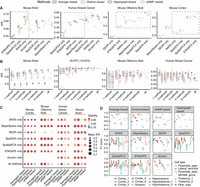
Comprehensive assessment of the accuracy and stability of four consensus strategies. (A) Consensus clustering results for four consensus strategies on seven baseline algorithms sorted from low to high according to average ARI. (B) Accuracies of four consensus strategies under different numbers of baseline algorithm. We randomly selected one to six baseline algorithms for mouse brain data, DLPFC sample 151672, and human breast data and selected one to five baseline algorithms for mouse olfactory bulb data and performed consensus clustering for each scenario 20 times. (C) Averaged ARI of four consensus strategies under “single method” and “all methods” situations. The size of the dots represents the mean ARI of 10 repeat experiments; color of the spots indicates stability. (D) Comparison of F1 scores across cell types for consensus strategies (top four panels) and baseline methods (bottom seven panels).
Next, we examined the impact of the number of baseline algorithms on the performance of consensus strategies on real SRT data sets. To this end, we randomly selected a subset of baseline algorithms (from one to six for mouse brain, sample 151672 of DLPFC, and human breast cancer data; from one to five for mouse olfactory bulb data) for consensus clustering and compared them with the full model that integrating all baseline algorithms. It can be seen that for normal tissues with a layered structure, namely, mouse brain, DLPFC, and mouse olfactory bulb data, the consensus performance increases with the number of baseline algorithms. The results of other samples of DLPFC data can be found in Supplemental Figure S17. However, the same phenomenon is not observed for data with scattered cell type distribution patterns such as human breast cancer data; namely, integration of one single baseline algorithm achieves near optimal clustering result (Fig. 4B).
We then thoroughly evaluated overall accuracy and stability of the four consensus strategies on real data with manual annotation as the ground truth, in which accuracy was measured by average ARI across 10 consensus results, and stability measures the consistency between 10 consensus results. Circle size in the figure signifies average ARI, with a larger circle indicating a higher value. Results consistently reveal that both average-based and hypergraph-based strategies exhibit the highest averaged ARI across all scenarios, followed by Onehot-based and wNMF-based strategies (Fig. 4C). Regarding stability, average-based and hypergraph-based consensus strategies exhibit the best resistance to randomness, whereas Onehot-based and wNMF-based strategies exhibit weaker stability (for the DLPFC data set, see Supplemental Fig. S18A,B).
To further evaluate the performance of different methods on a more detailed level, we examined the clustering accuracy at the cell type level (Mölbert and Haghverdi 2023), as measured by F1 score (Fig. 4D). Our consensus strategies demonstrated consistently high F1 scores across diverse cell populations, including both abundant and rare cell types. In contrast, baseline methods showed considerable variability in their performance. Although some baseline methods such as BayesSpace performed reasonably well for certain cell types, they often struggled with rare cell populations and regions with thin spatial layers. This cell type–level analysis reveals that our consensus approaches effectively overcome the limitations of individual methods, providing more reliable and consistent cell type identification across different cellular populations.
Based on the above analyses, we concluded that the four consensus strategies showed substantial differences in different data sets and scenarios. Average-based and hypergraph-based consensus strategies achieve high performance in integrating baseline algorithms and demonstrate superior accuracy and stability. The optimal number of baseline algorithms to be integrated should be determined by the cell type distribution pattern of the tissue sample. This nuanced evaluation guides appropriate consensus strategies given baseline algorithm and data characteristics across data sets.
Evaluation of consensus clustering strategies on the mouse cortex data set
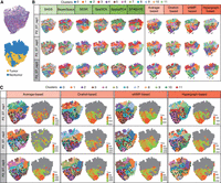
In this section, we applied STCC to the single-cell resolution mouse cortex data set generated by the STARmap technique (Wang et al. 2018). We focused on three consecutive tissue sections, BZ5, BZ9, and BZ14, that were assayed in the medial prefrontal cortex (mPFC) region of mice. These sections comprise 1049, 1053, and 1088 cells, respectively, each profiling the expression of the same set of 166 genes. The cells were annotated into 15 distinct cell types, including astrocytes (Astro), endothelial cells (Endo), and oligodendrocytes (Oligo), etc. We first compared the performance of four consensus strategies against individual baseline algorithms using the true number of clusters as input. Consistent with previous discoveries, the performance of consensus strategies is highly dependent on the selection of baseline algorithms. When using SEDR and SpaGCN as baselines, all four consensus strategies demonstrated significant advantages, outperforming the baselines across multiple evaluation metrics (Fig. 5A). In contrast, integrating SpatialPCA as a baseline algorithm improves clustering robustness but does not change the overall accuracy. For BASS, the average-based and Onehot-based consensus strategies surpass the baseline in terms of ARI, NMI, completeness score, and homogeneity score, whereas the hypergraph-based and wNMF-based strategies do not. No significant change in clustering accuracy is observed with BayesSpace and STAGATE as baseline algorithms (Fig. 5A). These results indicate the interplay between baseline methods and consensus strategies, highlighting the necessity to carefully select consensus strategies for STCC applications to real data sets.
Performance of consensus clustering strategies on the mouse cortex data. (A) Consensus clustering accuracy of the BZ5 sample of the mouse cortex data set based on a single baseline algorithm. Each baseline algorithm and consensus strategy were repeated 10 times. (B) Visualization of clustering results of the baseline algorithm (top) and four consensus strategies (bottom right) on the BZ5 sample of mouse cortex data. (C) UMAP visualization comparing ground-truth cell type labels (leftmost) with clustering results from four consensus strategies.
In practical applications, the true number of cell types is often unknown. To address this challenge, the STCC method is equipped to automatically determine the optimal number of clusters using a silhouette-based strategy, making it particularly suited for exploratory data sets in which the true number of clusters or spatial domains remains uncertain. Specifically, it calculates the silhouette score for a specified range of cluster numbers and selects the number with the highest score as the final cluster number. As indicated in Supplemental Figure S19A, the predicted cluster number (k = 14) with the maximal silhouette score closely approximates the true number (k = 15). These findings highlight the resilience of specific consensus strategies in maintaining clustering accuracy despite variations in the number of clusters, reinforcing their applicability in complex ST data sets.
Finally, we visualized the clustering results and performed trajectory inference. By taking the BZ5 slice as an example, all four consensus strategies successfully identified the hierarchical structures corresponding to the eL2/3 and eL6-1 cell types in the ground-truth annotations. In contrast, the baseline algorithms, especially BayesSpace, SEDR, SpatialPCA, and SpaGCN, exhibit more chaotic clustering in these regions, failing to display clear hierarchical structures (Fig. 5B). The UMAP embeddings demonstrate that all four consensus strategies effectively preserve the underlying cluster structures, with clear separation between different cell types that closely matches the ground-truth annotations (Fig. 5C). This dimensional reduction visualization further validates the robustness of our consensus approaches in capturing biologically meaningful cellular organizations. Clustering results for the other slices are shown in Supplemental Figures S20 and S21.
Consensus clustering and trajectory inference for the squamous cell carcinoma data
We further applied STCC to highly heterogeneous human squamous cell carcinoma (SCC) samples generated by the ST technique, which comprise 12 tissue sections from four patients. Following the method of Ji et al. (2020), we focused on three tissue sections from patient 2 as a representative example (Ji et al. 2020). Unlike previous data sets, this data set lacks detailed spatial domain annotations. Therefore, we used the histopathologist-annotated tumor and nontumor regions (P2_ST_rep2) as a silver standard for model evaluation (Fig. 6A).
Exploratory analysis of squamous cell carcinoma data. (A) Hematoxylin and eosin (H&E)–stained images (top) of squamous cell carcinoma samples, accompanied by corresponding rough annotations (bottom). (B) Spatial domain detection of six baseline algorithms and four consensus strategies in the analysis of squamous cell carcinoma patient 2. (C) Trajectory inference and pseudotime analysis of four consensus strategies in squamous cell carcinoma patient 2.
By incorporating the clustering results of six baseline methods as input, our consensus strategies effectively pinpoint the nontumor region at the lower part of each section (Fig. 6A). All four consensus strategies reveal clear structural patterns in this region (highlighted by black boxes), consistent with the coarse annotations. In contrast, the clustering results from the six baseline algorithms are highly scattered, lacking clear structure in the same region (Fig. 6B). Based on the clustering results from the consensus strategies, we next explored the differentiation relationship between tumor and nontumor regions. By inferring trajectories and pseudotime in this region, we identified a path tracing from nontumor regions toward tumor regions and found that the surrounded nontumor cells had a relatively earlier developmental time compared with the tumor cells (Fig. 6C). These findings provide valuable insights into the interconnectedness of the tumor region and neighboring regions, laying the foundation for a deeper understanding of tumorigenesis.
In summary, our consensus strategies provide valuable insights and robust support for downstream analyses compared with baseline methods, even for exploratory data sets in which the true number of cell types or spatial domains is unknown.
Discussion
The rapid accumulation of SRT data poses a great challenge for various downstream data analyses, especially for the most fundamental spatial domain detection step. Although a number of statistical or deep learning–based algorithms have been proposed for this task, there is no single algorithm that can achieve optimal results across all data sets. Consequently, there is an urgent need for a consensus framework that can harness the strengths of different algorithms to enhance clustering accuracy and stability. Although existing consensus frameworks such as SC3 and SAFE-clustering are designed specifically for scRNA-seq data, their performance on SRT data has not been tested. It is thus an important necessity to develop and evaluate different consensus strategies for SRT data, with a particular focus on their compatibility within different pipelines, platform dependence, accuracy, and efficiency when applied to SRT data.
To fill this gap, we proposed a scalable and flexible ST consensus framework called STCC. By integrating clustering results from both single and multiple baseline algorithms, STCC generally enhances clustering performance across diverse data sets and scenarios, particularly in cases in which baseline methods encounter challenges with complex spatial structures. The comprehensive analysis of the four consensus strategies highlights the preference for average-based consensus strategy, attributed to their simplicity, high accuracy, and stability. Notably, hypergraph-based exhibits exceptional stability and distinct advantages in the integration of vast data sets, wNMF-based underscores the enhancement in performance through consensus weighting. When it comes to the selection of consensus algorithms, we recommend (1) thoroughly exploring parameters of single baseline algorithm that could impact clustering results to attain the optimal consensus outcome, (2) adopting the more robust average-based and high effective hypergraph-based consensus strategies, and (3) selecting the appropriate number and type of baseline clustering algorithms based on the tissue origin of the samples.
Although demonstrating valuable results, our consensus framework still suffers from several limitations that should be addressed in future work. First, the current consensus framework takes only clustering outputs from baseline methods as input. It would be beneficial to explore the integration of various methods from the raw or processed data, such as the joint embedding from deep learning–based methods. This could potentially enhance the performance and robustness of the consensus clustering. Second, the current version of our consensus framework only incorporates seven tools, which is relatively limited considering the vast number of clustering tools currently available. To ensure a more robust consensus outcome, a broader range of clustering tools should also be incorporated into our consensus framework.
Methods
Baseline clustering algorithms for SRT data
We selected seven representative algorithms for spatial domain detection as the baseline algorithms for our consensus framework. Among them three are statistical based, namely, BASS (Li and Zhou 2022), BayesSpace (Zhao et al. 2021), and SpatialPCA (Shang and Zhou 2022), and four of them are deep learning based, namely, SEDR (Xu et al. 2024a), stLearn (Pham et al. 2023), SpaGCN (Hu et al. 2021), and STAGATE (Dong and Zhang 2022). These tools are widely used and highly recognized for the task of spatial domain detection. In detail,
-
BayesSpace is a Bayesian statistical method designed to enhance the resolution of SRT data and perform clustering by incorporating spatial neighborhood information as priors.
-
SpatialPCA is a spatially-aware dimensionality reduction method specifically designed for SRT data. Its core concept involves using the probabilistic PCA model to infer a low-dimensional representation of gene expression data while accounting for the underlying spatial correlation structure; thus, the inferred low-dimensional components are used for downstream analyses including spatial domain detection.
-
BASS is a Bayesian hierarchical model for simultaneous cell type and spatial domain detection across multiple scales and samples.
-
stLearn is a Python software package that utilizes histological image-derived morphological distances and spatial neighborhoods to smooth expression data to enable downstream analyses, such as spatial domain detection and trajectory inference.
-
SEDR is an autoencoder-based deep learning method that jointly captures low-dimensional embeddings of gene expression and spatial information in SRT data, which can be utilized for downstream analysis tasks such as clustering, trajectory inference, and batch effect correction.
-
SpaGCN is a graph convolutional network method to integrate multimodal data, including expression, spatial location, and histology to detect spatial domains.
-
STAGATE is a graph attention autoencoder to learn low-dimensional embeddings of SRT data by integrating gene expression and spatial information. The low-dimensional embedding can be utilized for spatial domain detection and denoising.
Simulated data for benchmarking consensus clustering algorithms
We conducted extensive simulations to evaluate the performance of the consensus strategies. The first simulation data (SimuData 1) is built from the mouse embryo data generated by Stereo-seq, with the purpose of investigating the impact of the number of spots on the runtime and maximum memory usage of consensus strategies. To achieve it, we downloaded the E12.5_E1S3 mouse embryo data from the MOSTA database, which comprises 49,908 spots quantitated by 17,337 genes, with a median gene count of 1237 per spot. We generated 15 data sets by randomly sampling a number of spots from this data set (with spot number ranging from 1000 to 15,000).
The second simulation data (SimuData 2) is obtained from mouse brain coronal data through the 10x Visium platform, which comprises 2688 spots measured on 18,078 genes (for details, see the next section). To investigate how the proportion of HVGs influences the performance of the consensus strategy, we identified 3000 HVGs using the “pp.highly_variable_genes” function in the SCANPY package (Wolf et al. 2018), leaving the remaining 15,078 genes as non-HVGs. We then created 11 data sets by combining varying numbers of HVGs with all non-HVGs, with the number of HVGs ranging from zero to 3000 in increments of 300. Analogy to SimuData 2, we constructed SimuData 3 by only replacing HVGs as SVGs inferred by “gr.spatial_autocorr” function from the Squidpy package (Palla et al. 2022).
Two additional simulation data sets (SimuData 4 and 5) are also based on the mouse brain coronal data. Among them, SimuData 4 is generated by adding random noises (with Gaussian distribution of mean zero and increasing standard deviations) on gene expression data, and SimuData 5 is constructed by selecting five to 20 cell types from all 20 annotated cell types to examine the impact of noise level and cell type number on the performance of the consensus strategy, respectively.
The final simulated data set (SimuData 6) was also constructed based on the mouse brain coronal data. It was designed to explore how the number of clusters specified in baseline algorithms affects the performance of various consensus strategies. We used cluster numbers ranging from five to 20 for the baseline algorithm SpaGCN, generating corresponding clustering results, which were then used as input for the consensus strategies.
For all above simulation data sets, we selected SpaGCN as the baseline algorithm and used its clustering outcome as input for different consensus strategies.
Real SRT data from different platforms for benchmarking consensus clustering algorithms
We downloaded seven publicly available SRT data sets with pathological annotation as gold standard to evaluate different consensus strategies. The first is the mouse brain coronal data mentioned in previous data simulation section. It spans various brain regions, encompassing 15 hierarchical structures including cortex, hippocampus, hypothalamus, and pyramidal layer. The second is human breast cancer data profiled by 10x Visium platform, which comprises 3798 spots and 36,601 genes, with a median gene count of 7943 per spot. This data set was manually annotated to 20 spatial regions, including DCIS/LCIS, IDC, tumor edge, and healthy regions. The third is human DLPFC (Maynard et al. 2021) measured on the 10x Visium platform. The data set comprises 12 tissue sections with 33,538 gene expression values from three adult donors. We acquired manually annotated labels for seven laminar clusters, including six cortical layers from L1 to L6 and the white matter (WM), as the gold standard for this data set, from the original publication. The fourth is the mouse olfactory bulb data (Rep11_MOB_ST) generated by ST technology (Xu et al. 2024b), which comprises 260 spots and 15,928 genes. Following the annotation, it is categorized into five hierarchical structures, namely, granular cell layer, mitral cell layer, outer plexiform layer, glomerular layer, and olfactory nerve layer. The fifth data set is the mouse cortex data obtained from online resources provided in the original study (Wang et al. 2018), comprising 1207 spots and 1020 genes. The data set is annotated into seven layers: corpus callosum (CC), hippocampus (HPC), layer 1 (L1), layer 2/3 (L2/3), layer 4 (L4), layer 5 (L5), and layer 6 (L6). Note that the fourth and fifth data sets did not include the necessary H&E images or other histological images required to run the stLearn algorithm. As a result, these two data sets do not contain the baseline results for the stLearn method. The sixth data set consists of three consecutive sections (BZ5, BZ9, BZ14) from the mouse cortex data, which measure the same set of 166 genes across 1049, 1053, and 1088 spots, respectively. Cells in this data set were annotated as 15 distinct cell types, including but not limited to Astro, Endo, and Oligo. The final data set was generated from human SCC using the ST technology. For this study, we downloaded three consecutive sections from patient 2. The data sets comprise 666, 646, and 638 spots, which measure the expression of 17,138, 17,344, and 17,883 genes, respectively. The detailed information of the above seven benchmark data sets is summarized in Figure 1B.
Overview of consensus strategies
Our proposed consensus strategies aim to integrate clustering results from diverse baseline algorithms, which can be represented as a hypergraph or a consensus matrix. The hypergraph matrix is generated by onehot encoding of each clustering result and concatenating them row-wise, in which a column corresponds to a clustering outcome of an algorithm for each spot/single cell and a row corresponds to a cluster. The consensus matrix is obtained by aggregating the connectivity matrices from individual clustering outputs, with each entry of the consensus matrix indicating the frequency of two spots assigning to the same cluster. Based on the obtained hypergraph and consensus matrices, the above four STCC consensus strategies can be elaborated as follows.
-
Onehot-based strategy simply applies k-means clustering to the hypergraph matrix to obtain consensus labels.
-
Average-based strategy applies k-means algorithm to the consensus matrix to derive consensus labels.
-
Hypergraph-based strategy employs hypergraph partitioning algorithms on the hypergraph matrix to derive consensus labels. We currently implemented three types of hypergraph partitioning algorithms, namely, hypergraph partitioning algorithm (HGPA), metaclustering algorithm (MCLA), and cluster-based similarity partitioning algorithm (CSPA). In detail, HGPA uses the weight of cutting hyperedges as the objective function to assess the partitioning quality of the hypergraph. MCLA first constructs a graph based on the hypergraph, with each node representing a spot and the weight of each edge measuring the number of times two spots being assigned to the same cluster. It then applies graph segmentation algorithm to partition it into categories to generate clustering labels. CSPA first computes similarities between hypergraphs (measured by Jaccard index) and then applies spectral clustering to the similarity matrix to obtain the final clustering result.
-
The wNMF-based consensus strategy assigns different weights to the connectivity matrices obtained from each baseline algorithm, that is,
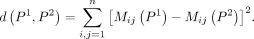
We define the binary connectivity matrix M(Pt) for the tth clustering result Pt, in which each element indicates whether two spots were assigned to the same cluster. In detail,
 where
where  and
and  are clustering labels of the spots i and j, respectively. The total number of spots is denoted by n.
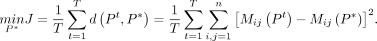
Based on the definition of the connectivity matrix, we define the distance between two clustering as
The goal of consensus clustering is to find the optimal clustering P* that is the closest to all clustering results obtained from individual baseline methods, which is defined under the following optimization objective:
Denote the consensus matrix as
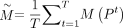 , and let
  . The objective function can then be rewritten as
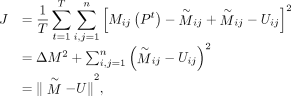 where
where  is a constant, and
  and U are matrices of
  and Uij, respectively.
The adjacency matrix U can be represented and constrained using a cluster indicator matrix
 , where Hij indicates whether sample j is assigned to cluster i, and k represents the number of clusters. This formulation allows us to express the consensus clustering solution as
  , which simplifies the optimization process and ensures the clustering constraints are satisfied. The consensus clustering
problem thus becomes
, which simplifies the optimization process and ensures the clustering constraints are satisfied. The consensus clustering
problem thus becomes 4.1
4.1
Given the definition of H,
 , where D is a k × k diagonal matrix. However, D is unknown until the problem is solved, so we eliminate D by defining
  . This leads to the following relations:
The final optimization problem is therefore transformed into a more tractable form:
The optimal values of
 and D can be calculated by the following multiplicative updating process in each iteration until convergence:
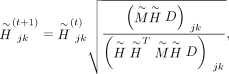
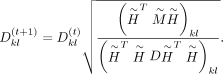
After solving for
 and D, the weighted consensus clustering problem transforms into the following optimization:
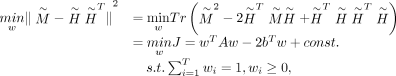 where
where  ,
, 
 .
.
Next, a quadratic programming algorithm is employed to iteratively solve for the optimal weights w. Finally, k-means clustering is applied to the weighted consensus matrix to derive the final consensus labels.
Cluster performance evaluation metrics
We employed seven metrics to evaluate the accuracy of the consensus clustering results.
-
Adjusted Rand index (ARI) is a similarity metric between two data partitions, often used for measuring clustering accuracy. It has a scale of −1 to 1, where a higher ARI indicates more precise clustering. ARI is calculated as
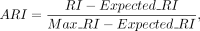 where RI is the original Rand index,
  is the expected RI under random assignment, and
  is the maximum RI value corresponding to completely correct clustering.
-
Normalized mutual information (NMI) is a measure of mutual dependence between two variables in information theory, defined as
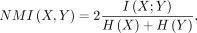 where I(X;Y) is the mutual information between X and Y, and H(.) is the Shannon entropy function.
-
Homogeneity is a measure for evaluating whether clusters contain data spots from a single true category, detailed as
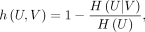 where H(U|V) is conditional entropy of the true category U given clustering V, and H(U) is Shannon entropy of U.
-
Completeness is a measure for measuring whether data spots from a true category are assigned to the same cluster. The equation is
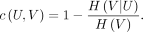
-
Calinski–Harabasz is an index measuring cluster dispersion ratios when true labels are unavailable. In detail,
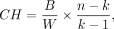 where B is the between-cluster variance, W is the within-cluster variance, n is the number of data spots, and k is the number of clusters.
-
Davies–Bouldin is an index evaluating average within-cluster distances against between-cluster distances without true labels. Given clusters Ci and Cj, the Davies–Bouldin index is calculated as follows:
 where Δ(Ci) is the intra-cluster distance, δ(Ci, Cj) is the inter-cluster distance, and k is the number of clusters. A lower Davies–Bouldin index indicates better clustering results.
-
Stability is an indicator for measuring the consistency of clustering results, defined as
 where nT is the number of all possible cluster pairs of T clustering results, and Ci and Cj represent the results of the ith and jth consensus clustering, respectively.
Pseudotime and trajectory analysis
Slingshot was used to perform trajectory inference and pseudotime analysis for the human SCC samples. It takes clustering labels as input and requires specification of the starting cluster to infer tissue-wide pseudotime trajectories. In our implementation, we specified the tumor region as the starting cluster to analyze the progression patterns from tumor to surrounding areas. The detailed workflow consists of the following steps:
-
Preparation of input data, including the clustering labels (clusterLabels) and dimensional reduction coordinates from our consensus clustering results;
-
Trajectory inference by Slingshot, which constructed a minimum spanning tree connecting clusters and fitted simultaneous principal curves to identify continuous trajectories;
-
Pseudotime calculation, which assigned pseudotime values to cells based on their position along the inferred trajectories, with cells in the tumor cluster designated as the starting point; and
-
Visualization using the plot_trajectory function to generate trajectory maps that integrate pseudotime information with spatial coordinates.
Data sets
All data analyzed in this article are available from publicly available data sets. The mouse brain and human breast cancer data sets are collected from 10x Genomics (https://support.10xgenomics.com/spatial-gene-expression/datasets). The DLPFC data set (Maynard et al. 2021) is accessible from the spatialLIBD package (https://github.com/LieberInstitute/HumanPilot). The ST data (Ståhl et al. 2016) for mouse olfactory bulb tissue is accessible from https://db.cngb.org/stomics/datasets/STDS0000017. The STARmap data (Wang et al. 2018) for mouse visual cortex is accessible on https://www.dropbox.com/sh/f7ebheru1lbz91s/AADm6D54GSEFXB1feRy6OSASa/visual_1020/20180505_BY3_kgenes?dl=0&subfolder_nav_tracking=1. The annotation information for STARmap data and the processed SCANPY object is provided at https://drive.google.com/drive/folders/1I1nxheWlc2RXSdiv24dex3YRaEh780my?usp=sharing. The processed data and manual annotations for STARmap data (Wang et al. 2018) across three consecutive sections of the mouse cortex are available at GitHub (https://github.com/zhengli09/BASS-Analysis/tree/master/data). The ST data for human SCC (Ji et al. 2020) are available under the NCBI Gene Expression Omnibus (GEO; https://www.ncbi.nlm.nih.gov/geo/) accession number GSE144240.
Software availability
The STCC framework is implemented in Python and has been made available on PyPI (https://pypi.org/project/STCC/). The source code for STCC is available at GitHub (https://github.com/hucongcong97/STCC) and as Supplemental Code.
Competing interest statement
The authors declare no competing interests.
Acknowledgments
This work was supported by the National Key R&D Program of China (2024YFC2309600 to X.Z., 2021YFC1712805 to H.-J.W.), National Natural Science Foundation of China (62372286 to X.Z., 32270683 and 32470662 to H.-J.W.), Science and Technology Innovation Plan of Shanghai (23JC1403200 to X.Z.), Beijing Natural Science Foundation (5242006 to H.-J.W.), and Fundamental Research Funds for the Central Universities (BMU2021YJ064 to H.-J.W. and PKU2022LCXQ027–Clinical Medicine Plus X–Young Scholars Project, Peking University). We acknowledge the bioinformatics core in the Center for Single-Cell Omics (CSCOmics), Shanghai Jiao Tong University School of Medicine, and the high-performance computing platform in Peking University for providing bioinformatics and high-performance computing services.
Author contributions: C.H. completed the data collection, conceptualization, and writing of the paper. X.Z. and H.-J.W. contributed to the conceptualization and writing of the paper. N.W. and J.Y. provided support during the paper revision process. All authors approved the final manuscript.
Footnotes
-
[Supplemental material is available for this article.]
-
Article published online before print. Article, supplemental material, and publication date are at https://www.genome.org/cgi/doi/10.1101/gr.280031.124.
- Received September 16, 2024.
- Accepted March 31, 2025.
This article is distributed exclusively by Cold Spring Harbor Laboratory Press for the first six months after the full-issue publication date (see https://genome.cshlp.org/site/misc/terms.xhtml). After six months, it is available under a Creative Commons License (Attribution-NonCommercial 4.0 International), as described at http://creativecommons.org/licenses/by-nc/4.0/.


