
Latent feature extraction with a prior-based self-attention framework for spatial transcriptomics
- 1Ministry of Education Key Laboratory of Bioinformatics, Bioinformatics Division at the Beijing National Research Center for Information Science and Technology, Center for Synthetic and Systems Biology, Department of Automation, Tsinghua University, Beijing 100084, China;
- 2School of Mathematical Sciences and LPMC, Nankai University, Tianjin 300071, China
Abstract
Rapid advances in spatial transcriptomics (ST) have revolutionized the interrogation of spatial heterogeneity and increase the demand for comprehensive methods to effectively characterize spatial domains. As a prerequisite for ST data analysis, spatial domain characterization is a crucial step for downstream analyses and biological implications. Here we propose a prior-based self-attention framework for spatial transcriptomics (PAST), a variational graph convolutional autoencoder for ST, which effectively integrates prior information via a Bayesian neural network, captures spatial patterns via a self-attention mechanism, and enables scalable application via a ripple walk sampler strategy. Through comprehensive experiments on data sets generated by different technologies, we show that PAST can effectively characterize spatial domains and facilitate various downstream analyses, including ST visualization, spatial trajectory inference and pseudotime analysis. Also, we highlight the advantages of PAST for multislice joint embedding and automatic annotation of spatial domains in newly sequenced ST data. Compared with existing methods, PAST is the first ST method that integrates reference data to analyze ST data. We anticipate that PAST will open up new avenues for researchers to decipher ST data with customized reference data, which expands the applicability of ST technology.
Recent innovations in spatially resolved transcriptomics grant us a novel perspective on the cellular transcriptome, and hence have stimulated efforts to unravel cell transcriptomes in the context of cellular organizations and catalyze new discoveries in different areas of biological research (Crosetto et al. 2015; Dries et al. 2021; Larsson et al. 2021; Zhuang 2021; Moses and Pachter 2022). Advanced spatial transcriptomic (ST) techniques, including Visium (10x Genomics), Slide-seq (Rodriques et al. 2019), and Stereo-seq (Chen et al. 2022a), could print spatially barcoded and oligo(dT) probes as microarrays of spots on the surface of glass slides, measuring genome-wide expression levels in captured locations, referred to as spots. When performing exploratory analysis of ST data, one of the most critical steps is characterizing spatial domains, which display spatially organized and functionally distinct anatomical structures on tissues. Nevertheless, low capture efficiency is one of the key reasons for high dropouts in single-cell RNA sequencing, leading to sparse and noisy data (Haque et al. 2017; Qiu 2020), and the limitations are also inherited by spatial transcriptomics data, making characterizing ST data computationally challenging (Zeng et al. 2022). Also, ST data usually represents substantial spatial correlation across tissues, requiring advanced approaches to take spatial localization information into account (Cheng et al. 2022; Zeng et al. 2022; Jiang et al. 2023).
Several computational methods have been proposed to analyze ST data (Dries et al. 2021; Cheng et al. 2022; Zeng et al. 2022). BayesSpace performs spatial clustering via modeling the spatial correlation of gene profiles between neighboring spots (Zhao et al. 2021). SpaGCN identifies spatial domains by integrating gene expression, spatial location and histology through the construction of an undirected weighted graph (Hu et al. 2021a). CCST is an unsupervised cell clustering method based on graph neural networks for ST data (Li et al. 2022). STAGATE integrates spatial information and gene profiles with an adaptive graph attention autoencoder to learn low-dimensional embeddings (Dong and Zhang 2022). DR-SC uses a hidden Markov random field to perform dimension reduction and spatial clustering within a unified framework (Liu et al. 2022b). Non-negative spatial factorization (NSF) is a spatially aware probabilistic dimension reduction method which assumes an exponentiated Gaussian process prior over the spatial locations (Townes and Engelhardt 2023). SpatialPCA integrates localization information with a kernel matrix and performs spatial-aware principle component analysis (PCA) for ST data (Shang and Zhou 2022). Also, SCANPY and Seurat, two widely-used single-cell analysis workflows in the Python and R communities, respectively, also provide vignettes tailored for ST data analysis (Wolf et al. 2018; Hao et al. 2021).
However, effective approaches for characterizing spatial domains in ST data need to overcome several challenges. First, existing methods failed to incorporate prior information from reference data to facilitate ST data analysis. Incorporating prior information in analyzing single-cell genomic data can better tackle the high level of noise and technical variation, and has been successfully applied in the analysis of various single-cell genomic data (Li et al. 2017; Lareau et al. 2019; Chen et al. 2021; Shengquan et al. 2021). With the advanced technologies, massive amounts of ST data have been generated by consortiums or individual research groups (Rodriques et al. 2019; Vickovic et al. 2019; Stickels et al. 2021) and accumulated in repositories and databases (Fan et al. 2020; Moses and Pachter 2022; Xu et al. 2022; Zeng et al. 2022; Yuan et al. 2023), paving the way to taking full advantage of the existing data and leveraging the data as reference to characterize spatial domains. Second, local spatial patterns should be effectively captured. Although it has been observed that aggregating information from each spot's neighbors via a graph convolutional network (GCN) is a promising approach to identify localized gene expression patterns (Hu et al. 2021a; Li et al. 2022; Zeng et al. 2022), tailored model design for better characterization of local spatial patterns is still demanded (Cheng et al. 2022). Third, global spatial patterns should be carefully preserved. With the exponential growth of profiled spots and genes, the graph-based approach becomes cumbersome and time-consuming, requiring strategies that perform memory and time-efficient minibatch training and prediction while preserving global spatial patterns. Fourth, there is an emerging need for the automatic annotation of spatial domains, because advanced protocols constantly increase sequencing throughput, and the typical approach, which performs unsupervised spatial clustering and then assigns the putative domain to each cluster subjectively, would be cumbersome and irreproducible for large-scale ST data.
To this end, we propose PAST, a Prior-based self-Attention framework for Spatial Transcriptomics, which incorporates the graph residual network (Zhang and Meng 2019; Liu et al. 2021) to effectively characterize spatial domains. PAST is a variational graph convolutional autoencoder, and uses a Bayesian neural network (BNN) (Blundell et al. 2015) to incorporate prior information from reference data, self-attention mechanism (Liu et al. 2021) to capture spatial patterns, and a ripple walk sampler (Bai et al. 2021) to enable scalable subgraph-based training and prediction. Featured as the first ST method which integrates reference data from various sources, PAST aims to extract latent embeddings of ST data in a self-supervised manner. The latent embeddings obtained from PAST contain valuable spatial correlation patterns and can be directly fed into existing scRNA-seq computational tools for effective and novel downstream analyses.
Results
Overview of PAST
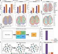
PAST is a self-supervised representation learning model based on a framework of variational graph convolutional autoencoder, taking transcriptomic profiles and spatial coordinates of the target ST data and transcriptomic profiles of the reference data as input. As shown in Figure 1B, the first layer of the encoder decomposes the total variation in ST data into two components (Li et al. 2017; Chen et al. 2021): the component that captures the shared biological variation from reference data based on the BNN module, and the component that captures the unique biological variation in target ST data based on an unconstrained fully connected network (FCN). The choice of the reference data is flexible and can be constructed from various sources (Fig. 1A; Supplemental Text S1), including: (1) external ST data of the same tissue and from the same protocol with the target ST data, (2) external ST data of similar tissues and from other protocols, (3) scRNA-seq data of similar tissues, or (4) the target ST data itself. In practice, the reference data can be incomplete: novel domains of biological variation that are not captured in the reference data can be present in target ST data. The second component uses an unconstrained FCN to adaptively capture the unique variation in target ST data that is not present in reference data.
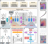
The PAST framework. (A) Four approaches for PAST to construct reference data, including three for external reference data (PAST-E) and one from the target data itself (PAST-S). (B) PAST is built on a variational graph convolutional autoencoder. The encoder of PAST consists of three layers, including the concatenation of a BNN and a FCN as the first layer and two self-attention modules as the subsequent two layers. The reparameterization module acquires the mean and log-variance matrix based on two FCNs, in which the mean matrix is the latent embedding obtained of PAST. The decoder of PAST is also a three-layer network, including a FCN layer and two stacked self-attention modules. The loss function of PAST consists of four parts, including reconstruction loss Lrecons, Kullback-Leibler divergence (KLD) loss Lkld, metric learning loss Lmetric and loss of BNN module Lbnn. (C) Ripple walk sampler samples high-quality subgraphs based on the spatial neighborhood graph and outputs minibatch gene expression matrices. (D) BNN module integrates shared biological variation through restricting the KLD distance between prior Gaussian distribution parameterized by reference data and Gaussian distribution parameterized by parameters of BNN. (E) The self-attention mechanism captures spatial correlation between neighbor spots, where FCN is used to generate queries, keys, and values for the calculation of attention weights. (F) The latent embeddings, that is, mean matrix in the reparameterization module, obtained by PAST facilitate various tasks including domain identification, trajectory inference, pseudotime analysis, multislice integration, and automatic annotation.
To integrate information of transcriptomic profiles and spatial coordinates, PAST identifies k-nearest neighbors (k-NN) for each spot using spatial coordinates in a Euclidean space, and adopts the graph residual network (Zhang and Meng 2019) with a self-attention mechanism (Liu et al. 2021) to aggregate information from each spot's neighbors. Specifically, the self-attention mechanism, which fits the relationship between words well in machine translation tasks (Raffel et al. 2020), is used to model local spatial patterns between neighboring spots, whereas the ripple walk sampler (Bai et al. 2021), which enables efficient subgraph-based training for large and deep GCNs, is used to achieve better scalability on large-scale ST data and preserve global spatial patterns simultaneously. PAST also restricts the distance of latent embeddings between neighbors through metric learning (Hadsell et al. 2006), the insight of which is that spatially close spots are more likely to be positive pairs to show similar latent patterns, illustrated in detail in the Loss function part of the Methods section. After model training and prediction, the latent embeddings, that is, the mean matrix of the reparameterization module (Fig. 1B), can be applied to spatial domain characterization, spatial visualization, trajectory inference, pseudotime analysis, multislice joint embedding, and automatic annotation (Fig. 1F).
PAST effectively leverages reference data from various sources for spatial domain characterization
We first use an example as a proof of concept to show the capability of PAST in incorporating reference data from different sources for spatial domain characterization. We collected ST data from a STARmap data set of the mouse primary visual cortex (MPVC) (Wang et al. 2018). We also constructed the reference data from the target ST data itself, a 10x Visium ST data set of the mouse brain coronal region (Palla et al. 2022), and a scRNA-seq data set of the mouse cortex (Tasic et al. 2016), which were referred to as PAST-S, PAST-E-Visium, and PAST-E-scRNA, respectively. The three variants of PAST were benchmarked against eight baseline methods, including two widely-used single-cell analysis workflows in Python and R community (SCANPY [Wolf et al. 2018] and Seurat [Hao et al. 2021]), and six methods for ST data analysis (SpaGCN [Hu et al. 2021a], CCST [Li et al. 2022], DR-SC [Liu et al. 2022b], NSF [Townes and Engelhardt 2023], SpatialPCA [Shang and Zhou 2022], and STAGATE [Dong and Zhang 2022]). We first show the advantages of PAST quantitatively from the following three perspectives. The detailed information about baseline methods and quantitative evaluation metrics are described in Supplemental Text S2.
First, we quantitatively evaluated the performance of spatial domain characterization via supervised cross-validation (Cross-validation). The supervised cross-validation aims to assess the representation capabilities of the latent embeddings learned by various methods. Specifically, we treated the latent embeddings as the input and the labels of spatial domains as the output, adopted support vector machine (SVM) as the classifier as suggested by a benchmark study on supervised single-cell annotation (Abdelaal et al. 2019), and conducted fivefold cross-validation experiments. We evaluated the performance by the average score of accuracy (Acc), Cohen's kappa value (κ), mean F1 score (mF1), and weighted F1 score (wF1), respectively, in the fivefold experiments. A higher score of the metrics suggests that the latent embeddings can better predict the spatial domains and, consequently, have superior representation capabilities. As shown in Figure 2A and Supplemental Figure S1A, except SpatialPCA, PAST-S and PAST-E-Visium outperform the remaining seven baseline methods for excellent embedding capabilities. Although PAST-E-scRNA performed worse than SpatialPCA and STAGATE, which may be caused by the inconsistency of tissues and protocols between ST data and the reference scRNA-seq data, it still outperforms the other six baseline methods. To qualitatively evaluate the representation capabilities of low-dimensional embeddings, we also visualized the spots using uniform manifold approximation and projection (UMAP) and t-distributed stochastic neighbor embedding (t-SNE) based on the latent embeddings learned by different methods (Fig. 2B; Supplemental Fig. S2A). Except L2/3, L6, and CC, SCANPY and Seurat could hardly distinguish other domains. SpaGCN, DR-SC, NSF provide relatively better performance. STAGATE succeeded to detect most of the domains but still failed to decipher the heterogeneity of HPC. The three variants of PAST consistently achieve satisfactory visualization results compared with other methods and only SpatialPCA, PAST-S, and PAST-E-Visium successfully distinguished HPC from other domains.
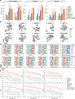
PAST effectively leverages reference data from various sources for spatial domain characterization. (A) Quantitative performance evaluation of spatial domain characterization on STARmap MPVC data set via supervised cross-validation and unsupervised spatial clustering with a specified number of clusters (Ncluster) and with default resolution (Dlouvain). The cross-validation performance was evaluated by the average score of Cohen's kappa value (κ) and mean F1 score (mF1), respectively, in the fivefold experiments. The spatial clustering performance was evaluated by adjusted rand index (ARI) and adjusted mutual information (AMI). (B) UMAP visualization results, (C) spatial visualization of clustering with a specified number of clusters and the manual annotation and (D) clustering evaluation of different methods under various dropout rates on MPVC data set.
Second, we compared the performance of spatial domain characterization through the unsupervised spatial clustering with a specified number of clusters (Ncluster), in which the specified number of clusters is set to the number of unique ground-truth spatial domains. We directly used the baseline spatial clustering methods, such as CCST (Li et al. 2022) and SpaGCN (Hu et al. 2021a), or the accompanying spatial clustering strategy of each of the other baseline methods on the learned latent embeddings. Following STAGATE, PAST performed clustering with a specified number of clusters by the mclust algorithm. For SCANPY, Seurat and NSF which perform clustering by Louvain or Leiden, we implemented a binary search to tune the resolution parameter in clustering to make the number of clusters and the specified number as close as possible. We evaluated the clustering performance by six metrics: adjusted rand index (ARI), adjusted mutual information (AMI), normalized mutual information (NMI), Fowlkes-Mallows index (FMI), completeness (Comp), and homogeneity (Homo). As shown in Figure 2A and Supplemental Figure S1A, PAST-S and PAST-E-Visium provide superior performance than all eight baseline methods on all six metrics. PAST-E-scRNA only performs slightly worse than SpatialPCA even when integrating incompatible scRNA-seq data as reference. SCANPY and Seurat, two widely-used single-cell analysis workflows, provided a relatively poor performance even using the vignettes tailored for ST data, indicating the importance of utilizing spatial information. Furthermore, visualization of the spatial domains characterized by clustering with a specified number of clusters and the ground-truth spatial domains on the spatial coordinates of ST data also show consistent results with the quantitative evaluation (Fig. 2C). Note that for CCST, we only evaluated the clustering performance with a specified number of clusters because it is a spatial clustering method and does not provide latent embeddings.
Third, we test the performance of PAST and other methods for the unsupervised spatial clustering with default resolution (Dlouvain), which is useful for the general situation in which the number of unique ground-truth spatial domains is unknown (Cheng et al. 2022). We performed Louvain clustering algorithm, one of the most widely-used community-based clustering methods in single-cell studies, with default resolution based on the latent embeddings learned by different methods. As shown in Figure 2A and Supplemental Figure S1A, PAST-S again achieves overall the best performance whereas PAST-E-Visium and PAST-E-scRNA perform better than any other baseline methods except SpatialPCA. It is vital to emphasize that PAST-scRNA, which incorporates scRNA-seq data to analyze ST data, even achieved 28.2% and 32.0% improvement compared to a competitive ST method STAGATE in terms of ARI and AMI, respectively (31.6%, 18.3%, 29.1%, 34.1% for NMI, FMI, Comp, and Homo, respectively). The evaluation results are detailed in Supplemental Table S1.
To mimic protocols that provide low coverage, we down sampled the reads in the target ST data by randomly dropping out the entries in the expression matrix to zero with a probability equal to the specified dropout rate, as suggested by a recent benchmark study (Cheng et al. 2022). As shown in Figure 2D, all methods including the three variants of PAST were affected by the increase in the dropout rate, however, PAST with external reference (i.e., PAST-E-Visium and PAST-E-scRNA) consistently outperform the remaining methods over all different dropout rates. Altogether, the results above suggest PAST effectively deciphers spatial patterns through integrating external reference data constructed from various sources and when target ST data has a higher degree of sparsity and noise, the benefit of utilizing external reference data increases. Furthermore, we also showed that PAST is robust to model hyperparameters including the number of neighbors and latent dimensions on the STARmap MPVC data set (Supplemental Figs. S3, S4).
PAST robustly obtains informative low-dimensional embeddings and facilitates diverse downstream analyses
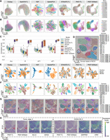
To test the capability of PAST in learning effective embeddings and accomplishing downstream tasks, we further collected 12 human dorsolateral prefrontal cortex (DLPFC) slices from a 10x Visium data set (Maynard et al. 2021). For each slice, we constructed the reference data from the ST data itself and from external ST data, namely the remaining 11 slices. The two variants of PAST have different application scenarios and are referred to as PAST-S and PAST-E, respectively. First, we benchmarked PAST from the three quantitative perspectives against nine baseline methods, including the eight methods tested on the STARmap MPVC data set and a clustering method specifically designed for spatial transcriptomics (Ståhl et al. 2016) and 10x Visium data, namely BayesSpace (Zhao et al. 2021). Similar to CCST, we only evaluated the clustering performance with a specified number of clusters. As shown in Figure 3A and Supplemental Figure S5A, for supervised cross-validation, PAST-S and PAST-E performs better than other five baseline methods except NSF and SpatialPCA. Furthermore, PAST-S and PAST-E outperforms all the baseline methods in terms of unsupervised spatial clustering with a specified number of clusters and unsupervised spatial clustering with default resolution on the 12 DLPFC slices (Supplemental Table S2). One-sided paired Wilcoxon signed-rank tests showed that PAST-E showed much more advantages than PAST-S in terms of various clustering metrics in the two different clustering scenarios, with P-values of 0.0105 and 0.0002 for ARI, respectively (0.0061 and 0.0002 for AMI, 0.0061 and 0.0002 for NMI, 0.0105 and 0.0005 for FMI, 0.0105 and 0.0002 for Comp, and 0.0134 and 0.0002 for Homo), highlighting the benefit of integrating high-quality external reference data. Similarly, we visualized the spatial domains characterized by clustering with a specified number of clusters and the ground-truth spatial domains on the spatial coordinates of ST data to qualitatively evaluate the performance of different methods (Supplemental Fig. S6). Taking Slice 151,673 as an example, the spatial domain assignment of the nonspatial approaches, namely SCANPY and Seurat, provide poor continuity and smoothness, which is consistent with the above quantitative results. SpaGCN, NSF, and BayesSpace fail to decipher the expected layer pattern in layer 4–layer 6 of this slice, which impairs the spatial clustering accuracy, whereas CCST, DR-SC, SpatialPCA, STAGATE, PAST-S, and PAST-E successfully characterized the expected cortical layer structures, indicating the effective spatial domain characterization.
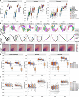
PAST robustly obtains informative low-dimensional embeddings and facilitates diverse downstream analyses. (A) Quantitative performance evaluation of spatial domain characterization on 12 DLPFC slices via supervised cross-validation and unsupervised spatial clustering with a specified number of clusters (Ncluster) and with default resolution (Dlouvain). The cross-validation performance was evaluated by the average score of Cohen's kappa value (κ) and mean F1 score (mF1), respectively, in the fivefold experiments. The spatial clustering performance was evaluated by adjusted rand index (ARI) and adjusted mutual information (AMI). The center line, box limits and whiskers in the boxplots are the median, upper and lower quartiles, and 1.5× interquartile range, respectively. (B) UMAP visualization, (C) PAGA trajectory inference results, and (D) DPT pseudotime analysis results of Slice 151,673. (E) The number of shared spatial domains in external reference data gradually deceased. (F) The spots in external reference data of PAST were down sampled with a stratified random sampling strategy to construct reference data with various scales. The horizontal dashed lines represent the corresponding median scores of STAGATE.
Second, taking Slice 151,673 as an example, we performed various downstream analyses based on the low-dimensional embeddings obtained by different methods. For low-dimensional visualization based on the UMAP and t-SNE algorithm (Fig. 3B; Supplemental Figs. S7, S8), except the white matter (WM), SCANPY and Seurat could hardly distinguish the cortical layers. SpaGCN DR-SC, and NSF provided relatively better performance, whereas SpatialPCA, STAGATE, PAST-S, and PAST-E successfully identified all the spatial structures and reconstructed the manifold of them. Also, UMAP and t-SNE visualization for the other 11 DLPFC slices provided similar results (Supplemental Figs. S7, S8). For spatial trajectory inference, based on the latent embeddings learned by different methods, we performed trajectory inference using PAGA on Slice 151,673 (Wolf et al. 2019). As shown in Figure 3C, PAST captured the well-known corticogenesis patterns (Gilmore and Herrup 1997; Agirman et al. 2017) and inferred a nearly linear development trajectory from inner to outer layers, indicating the utility of PAST in revealing development trajectory. For spatial pseudotime analysis using the DPT algorithm (Haghverdi et al. 2016), PAST successfully characterized all the continuous development stages, whereas the other baseline methods only captured the pseudotime variation between WM and other cortical layers (Fig. 3D). Trajectory inference and pseudotime analysis for other slices also provided similar results (Supplemental Figs. S9, S10), highlighting the potential of PAST to extract informative features and facilitate downstream analyses and biological implications. The detailed implementation of visualization, clustering and other downstream analyses are shown in Supplemental Text S3.
The previous example on DLPFC slices used external reference data constructed from the other slices, which contains more than 40,000 spots and heterogeneous information of almost all the domains (PAST-E). However, the prior information in external reference data is generally incomplete for the target ST data and the scale of high-quality reference data is generally limited. Therefore, we further carefully examined the robustness of PAST-E to the number of shared domains and scale of reference data, using STAGATE, a competitive method on DLPFC data set, as the baseline. We gradually left out different number of spatial domains in external reference data, and obtained PAST-E-LO1, PAST-E-LO2, PAST-E-LO3, and PAST-E-LO4, which denote leaving out layer 1, layers 1 and layer 2, layers 1 through layer 3, and layers 1 through layer 4, respectively. The results shown in Figure 3E and Supplemental Figure S11A were in line with intuition because as the spatial domains are continuously left out, the effective prior information in the reference data is decreased. Except PAST-E-LO4, the overall clustering performance of PAST-E when integrating reference with different number of shared domains is superior to STAGATE (the horizontal dashed lines), and PAST-E performs well even based on the reference data containing only nearly half of shared domains. Furthermore, another two different schedules removing the same number of shared domains in external reference data obtained similar results (shown in Supplemental Figs. S12, S13), suggesting the robustness of PAST to the number of shared domains in reference data. Meanwhile, to test the influence of limited scale of reference data without reducing the number of shared domains, we randomly down sampled the spots in reference data based on a stratified random sampling strategy, that is, sampling spots from each domain with a given rate. We obtained PAST-E-DS50, PAST-E-DS40, PAST-E-DS30, PAST-E-DS20, PAST-E-DS10, PAST-E-DS5, and PAST-E-DS1, which denote remaining sampled 50%, 40%, 30%, 20%, 10%, 5%, and 1% of the spots, respectively. Compared with PAST-E which integrated prior information from more than 40,000 spots, the data scale of reference of PAST-E-DS50 through PAST-E-DS1 was only 21,949 through 425. As shown in Figure 3F and Supplemental Figure S11B, PAST-E with down sampled reference data consistently achieves satisfactory performance for supervised cross-validation and spatial clustering, until only 1% of the spots in reference data remained. We then performed two-sided Wilcoxon signed-rank tests on the quantitative results of different reference data scales. As shown in Supplemental Figure S14, the scale of reference data, which may range from a few hundred to tens of thousands, has no significant impact on the performance of PAST-E, indicating that PAST-E is highly robust to the data scale of reference data when the number of shared domains in reference is sufficient.
PAST captures local spatial patterns with self-attention mechanism
Next, we tested whether PAST could provide insights into local spatial patterns. We applied PAST to an osmFISH mouse somatosensory cortex data set (MSC) (Codeluppi et al. 2018), and used the target data itself as reference. As shown in Figure 4A and Supplemental Figure S15, PAST-S effectively characterizes spatial domains, and achieves significant improvement compared to the baseline methods in terms of cross-validation, and spatial clustering with a specified number of clusters or with default resolution (Supplemental Table S3). Also, PAST with different numbers of neighbors also showed its consistent superiority (Supplemental Fig. S16). For spatial visualization, PAST-S successfully identifies the expected structures and delineated the layer borders clearly, and the identified domains are more consistent with the original annotation of the data set (Fig. 4B,C).
PAST capably captures local spatial patterns with self-attention mechanism. (A) Quantitative performance evaluation of spatial domain characterization on the osmFISH MSC data set via supervised cross-validation and unsupervised spatial clustering with a specified number of clusters (Ncluster) and with default resolution (Dlouvain). The cross-validation performance was evaluated by the average score of Cohen's kappa value (κ) and mean F1 score (mF1), respectively, in the fivefold experiments. The spatial clustering performance was evaluated by adjusted rand index (ARI) and adjusted mutual information (AMI). (B) Visualization of the results of spatial clustering with a specified number of clusters on MSC. (C) The manual annotation of MSC. (D) UMAP visualization of spots in MSC. The blue, orange, and brown circles denote Layer 2–3 lateral, Layer 2–3 medial, and ventricle, respectively. (E) The neighbor proportion and attention proportion for border spots of domains Layer 2–3 lateral, Layer 2–3 medial, and ventricle, respectively.
We then explored the capability of the self-attention module of PAST-S in capturing local spatial patterns. As shown in Figure 4D and Supplemental Figure S17, compared with baseline methods like SCANPY, Seurat, DR-S,C and SpaGCN, PAST could effectively identify domains like Layer 2–3 lateral, Layer 2–3 medial, and ventricle in UMAP and t-SNE visualization (blue, orange, and brown circles). For these three spatial domains, we selected the border spots whose spatial neighbors were originated from at least one other spatial domain, and calculated the neighbor proportion and attention proportion of each domain. More specifically, for each border spot of each domain, we recorded the proportion of different spatial domains in the six nearest neighboring spots, and calculated the average proportion for all the border spots of each domain, resulting in the neighbor proportion. In comparison with the neighbor proportion, the attention proportion recorded the attention-weighted proportion of different spatial domains in the six nearest neighboring spots. As shown in Figure 4E, the self-attention mechanism successfully identifies the neighboring spots from the same domain and improves the corresponding weights, that is, from 70.15% to 72.14% for Layer 2–3 lateral, from 72.41% to 75.92% for Layer 2–3 medial, and from 72.77% to 80.45% for ventricle, indicating that self-attention mechanism enables border spots to aggregate more information from neighbor spots belonging to the same domain. Taken together, PAST could effectively capture the local spatial patterns with the self-attention mechanism and characterize the spatial correlation of the spots in ST data, especially the easily confused border spots.
PAST enables scalable training and prediction on large data while preserving global spatial patterns
With the development of ST technologies, the number of profiled spots and genes increases exponentially, requiring the scalability of computational methods. Traditional minibatch training strategy for deep learning, which partition entire data set into minibatches based on random sampling, is not suitable for graph neural network (GNN) because of the destruction to the connectivity and structure of graph (Bai et al. 2021; Zeng et al. 2022), making GNN-based methods such as SpaGCN (Hu et al. 2021a) and CCST (Li et al. 2022) not applicable to large-scale ST data. STAGATE partitioned the profiled slice and constructed a graph for each part to enable training on large data (Fig. 5D), which may lead to the loss of global spatial patterns (Dong and Zhang 2022). We thus introduced a subgraph-based strategy for scalable training and prediction that considers both the randomness and connectivity of the graph and samples high-quality subgraphs based on a ripple walk sampler (RWS). RWS was originally proposed only for training, and was extended by us from training to prediction by sampling subgraphs covering all spots of the target data set and aggregating the latent embeddings of different subgraphs in an ensemble manner (Methods). Based on the RWS strategy, PAST preserves global spatial patterns and enables efficient application simultaneously.
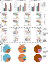
PAST enables scalable training and prediction on large data while preserving global spatial patterns. (A) Quantitative performance evaluation of spatial domain characterization on the Stereo-seq MOBS1 data set via supervised cross-validation and unsupervised spatial clustering with a specified number of clusters (Ncluster) and with default resolution (Dlouvain). The cross-validation performance was evaluated by the average score of Cohen's kappa value (κ) and mean F1 score (mF1), respectively, in the fivefold experiments. The spatial clustering performance was evaluated by adjusted rand index (ARI) and adjusted mutual information (AMI). (B) The manual annotation of MOBS1. (C) Visualization of the results of spatial clustering with a specified number of clusters on MOBS1. (D) Sampling strategy of STAGATE for minibatch training. (E) Ripple walk sampling strategy of PAST for scalable subgraph-based training and prediction. (F) Average time cost of different methods on MOBS1. (G) Peak memory usage of different methods on MOBS1.
We collected a Stereo-seq mouse olfactory bulb section (MOBS1) with 107,416 spots and 26,145 genes and analyzed the data set on a standard desktop with an AMD Ryzen 7 Eight-Core 3800X CPU, 64GB of RAM and an NVIDIA GeForce RTX 2080 Ti GPU. We collected another Stereo-seq mouse olfactory bulb section (MOBS2) with 104,931 spots and 23,815 genes to construct the external reference for PAST. Note that we encountered memory errors when performing Seurat, SpaGCN, CCST, NSF, and SpatialPCA on MOBS1. As shown in Figure 5A and Supplemental Figure S18, PAST-S and PAST-E, which incorporated self-prior information from MOBS1 itself and external-prior information from MOBS2, respectively, achieve overall the best performance for spatial domain characterization. The quantitative results are listed in Supplemental Table S4. Furthermore, PAST-S and PAST-E also achieve satisfactory performance in UMAP and t-SNE visualization (Supplemental Fig. S19). Also, the spatial domains detected by PAST-S and PAST-E were spatially continuous and smooth, and the subependymal zone (SEZ) domain, denoted as Cluster 1, was only successfully characterized by these two variants of PAST (Fig. 5B,C). We performed differential expression gene (DEG) analysis for Cluster 1 of PAST-S and PAST-E, respectively. The results of both of these two variants showed that the top two DEGs were Mbp and Plp1, which are classical genes encoding myelin proteins (Bitar et al. 2022). Myelin proteins were usually used as markers for striatal contamination or staining to facilitate accurate dissection of the SEZ (Friess et al. 2021; Bitar et al. 2022). We further performed Gene Ontology (GO) analysis for the top 10 DEGs with the lowest adjusted P-values of Cluster 1, and identified the most significant molecular function, that is, structural constituent of myelin sheath, with false discovery rates (FDR) of 1.28 × 10⁻⁴ and 9.33 × 10⁻⁵ for PAST-S and PAST-E, respectively. The GO analysis results were well consistent with the molecular function of SEZ domain, that is, deriving oligodendrocytes to form mature myelin sheaths around axons (Menn et al. 2006; Kazanis 2009), suggesting the ability of PAST to facilitate functional implication.
We also recorded the computational time and peak memory usage of different methods, especially the two GNN-based methods, that is, STAGATE and PAST, which used different sampling strategies (Fig. 5D,E). As shown in Figure 5F, the average computational time of PAST-S and PAST-E (168 and 164 sec) in 10 replicated experiments were approximately 30× less than STAGATE (5304 sec). In terms of peak memory usage, PAST-S and PAST-E also consumed significantly less memory than STAGATE (Fig. 5G), indicating that the RWS of PAST has a significant advantage over the partition strategy of STAGATE. SCANPY adopts the straightforward representation learning methods, that is, principle component analysis, without incorporating spatial information of ST data, thus providing relatively inferior performance but consuming the lowest computation time (26 Sec). In summary, PAST enables scalable subgraph-based training and prediction while preserving global spatial patterns to better characterize spatial organizations.
PAST facilitates multislice joint embedding and automatic domain annotation
Advanced ST sequencing technologies like 10x Visium, Slide-seq (Rodriques et al. 2019), Slide-seq v2 (Stickels et al. 2021), and Stereo-seq (Chen et al. 2022a) generate multiple sequencing slices for the same tissue at one time. However, because of the difference in the dissection of the tissue slices and their placement on array, the spatial coordinate system of multiple slices are different and cannot be easily compared across slices (Zeira et al. 2022), urgently requiring computational methods for multislice joint embedding and automatic domain annotation. We hence proposed two strategies, namely a transfer learning (TL) strategy and a three-dimensional (3D) stacking (3DStack) strategy, based on current representation learning framework to acquire joint embeddings of multiple slices (Supplemental Text S4). Specifically, given multiple slices with inconsistent coordinates and a deep representation learning model, TL strategy chooses one among these slices to train the deep representation learning model and then acquires the joint embeddings of all slices based on the trained model. In comparison, the 3D stacking strategy adds a third dimension to stack the multiple slices in a 3D space and only considers spatial relationship between spots from the same slice by setting the distance between different slices to a large value (Supplemental Fig. S20). Based on the 3D coordinates reconstructed by 3D stacking strategy, current representation learning methods can be easily applied to multiple slices for joint embedding. After obtaining joint embeddings of multiple slices, automatic domain annotation can be easily implemented with a specified classifier (Supplemental Text S4). Specifically, we first split the data into a reference set with domain labels and a target set without labels, then based on the joint embeddings, we trained a SVM on the reference set with its embeddings and labels, and predicted the labels of target set with the trained SVM. Note that the official implementation of DR-SC, SpaGCN, SpatialPCA, and STAGATE cannot use 3D coordinates, whereas SCANPYand Seurat cannot integrate spatial information, thus not applicable to 3D stacking strategy. Nondeep learning models like SCANPY, Seurat, NSF, DR-SC and SpatialPCA are not applicable to TL strategy designed for deep methods, and acquire the latent embeddings of each slice separately in the subsequent experiments.
We first adopted the 12 DLPFC slices to quantitatively show the integration and annotation performance of different methods based on the two strategies, denoting methods using the TL and 3DStack strategies as *-TL and *-3DStack, respectively. We split the DLPFC data set into a reference set, that is, Slice 151,673 with domain labels, and a target set, that is, remaining slices without labels. Naturally, PAST constructed reference data of the BNN module using Slice 151,673 with domain labels. As the UMAP and t-SNE visualization shown in Figure 6A,B and Supplemental Figure S21A–C, methods like SCANPY, Seurat, NSF, DR-SC, and SpatialPCA, which were directly applied to multiple slices and acquired the latent embeddings separately, obtain relatively poor performance, whereas STAGATE-TL, PAST-TL, and PAST-3DStack succeed in batch correction and domain identification, based on the joint embeddings of all the 12 slices obtained by TL and 3DStack strategy. We next used the embeddings and domain labels of Slice 151,673 to train a SVM classifier and annotated the spatial domains in other slices. For quantitative comparison of annotation results, PAST-TL consistently outperforms the baseline methods (Fig. 6C), and achieved significantly higher scores of Acc, κ, mF1, and wF1 than STAGATE-TL, the second-best method, with P-values of 0.0034, 0.0024, 0.0005, and 0.0005, respectively, in one-sided paired Wilcoxon signed-rank tests. PAST based on the 3D stacking strategy, namely PAST-3DStack, provides even better performance than PAST-TL and naturally outperforms any other baseline methods. Furthermore, clustering evaluation of the joint embeddings showed similar results (Supplemental Fig. S21D), highlighting the superiority of the TL and 3DStack strategies and PAST in multislice integration and automatic annotation.
PAST facilitates multislice joint embedding and automatic domain annotation. UMAP visualization of spots based on the joint embeddings of all the 12 DLPFC slices colored by (A) slices and (B) spatial domains. (C) Performance of supervised annotation evaluated by accuracy (Acc), Cohen's kappa value (κ), mean F1 score (mF1), and weighted F1 score (wF1), where Slice 151,673 was taken as the training set and other 11 slices were taken as test sets. The center line, box limits, and whiskers in the boxplots are the median, upper and lower quartiles, and 1.5× interquartile range, respectively. (D) The manual annotation of BCS1, in which the IDC_3 tumor region was black circled. UMAP visualization of the joint embeddings of spots in BCS1/2 sections colored by (E) sections and (F) spatial domains. (G) The supervised annotation results on BCS2 by different methods. The black circle denotes the supervised annotated IDC_3 and Tumor_edge_3, whereas the blue and orange circles denote the supervised annotated DCIS/LCIS_1 and DCIS/LCIS_2, respectively. (H) The annotation results of Tumor_edge_3 and DCIS/LCIS_2 by PAST-TL and PAST-3DStack and the spatial expression patterns of BCS1-marker genes on BCS2.
We further collected another two 10x Visium human breast cancer sections (BCSs) for integration and annotation, where the first section (BCS1) of the data set is precisely annotated by (Fu et al. 2021) and the second section (BCS2) is not annotated. Naturally, we treated BCS1 (Fig. 6D) as reference set with domain labels and treated BCS2 as target set for annotation. PAST-TL and PAST-3DStack again successfully correct the batch effect between the sections and separate spots from different domains (Fig. 6E,F; Supplemental Fig. S22A,B,D). Based on joint embeddings acquired by different methods, we next trained a SVM classifier with embeddings and labels of BCS1, and annotated BCS2 (Fig. 6G; Supplemental Fig. S22C). For the evaluation of annotation results, we identified marker genes for each domain based on the ground-truth labels on BCS1 (referred to as BCS1-marker genes), and found that BCS1-marker genes of each domain were also differentially expressed in most of the corresponding PAST-TL and PAST-3DStack annotated tumor areas on BCS2 (Supplemental Fig. S23), indicating the ability of PAST-TL and PAST-3DStack to reveal biological variation among tumor areas. In addition, PAST successfully captured BCS2-specific spatial domains by separating the IDC_3 region on BCS1 into IDC_3 and Tumor_edge_3 on BCS2 (black circles in Fig. 6D,G). The BCS1-marker genes of Tumor_edge_3 also showed the unique spatial pattern of the newly annotated Tumor_edge_3 on BCS2, which further suggests the accuracy of annotation results on BCS2 (Fig. 6H). We also performed DEG analysis for Tumor_edge_3 region based on the annotation results of PAST-TL and PAST-3DStack on BCS2, and identified the same five most significant DEGs including IGHG3, IGKC, IGLC2, IGHG4, and IGHG1 with adjusted P-values of 1.11 × 10−83, 1.86 × 10−78, 9.18 × 10−74, 9.18 × 10−74, 1.66 × 10−69 for PAST-TL and 4.52 × 10−74, 2.60 × 10−69, 8.11 × 10−66, 1.75 × 10−62, 3.21 × 10−60 for PAST-3DStack, respectively. Based on previous literature, the linkage of IGHG1/3/4 provides information for prognosis of diseases like autoimmunity and malignancy (Oxelius and Pandey 2013), IGKC, serving as a robust immune marker, could predict metastasis-free survival and response to chemotherapy (Schmidt et al. 2012), and IGLC2 was proven to be a significant prognostic biomarker for triple-negative breast cancer patients (Chang et al. 2021). The Gene Ontology enrichment for the top 10 DEGs of Tumor_edge_3 also significantly revealed lots of biological immune processes for both PAST-TL (Supplemental Fig. S24) and PAST-3DStack model (Supplemental Fig. S25).
PAST-TL and PAST-3DStack also successfully captured the biological difference between DCIS/LCIS_1 and DCIS/LCIS_2 (blue and orange circles in Fig. 6G) and accurately annotated DCIS/LCIS_2 on BCS2, which was missed by other methods. The spatial expression visualization of BCS1-marker genes of DCIS/LCIS_2 on BCS2 illustrated the accurate annotation of DCIS/LCIS_2 by PAST and the two strategies (Fig. 6H). To summarize, based on the two strategies, PAST cannot only effectively facilitate multislice joint embedding and automatic domain annotation, but also identify test set-specific spatial patterns and reveal the corresponding biological implications.
Discussion
In this article, we introduce PAST, a comprehensive and scalable framework that effectively integrates prior information via Bayesian neural networks, deciphers global and local spatial correlations based on graph residual network integrated with self-attention mechanism, and enables scalable training and prediction on large data sets with RWS strategy. With comprehensive experiments on multiple data sets generated by various technologies, we have shown that PAST capably incorporates prior information from various sources to better tackle the high-level technical variation and effectively integrates spatial information to characterize spatial domains, highlighting the superior information fusion capabilities of PAST. We have also showed the successful applications of PAST in downstream tasks including spatial domain characterization, ST visualization, spatial trajectory inference, and pseudotime analysis. Experiments on large-scale data sets also proved the scalability and effectiveness of PAST. Furthermore, PAST not only enables multislice joint embedding and automatic annotation of spatial domains for multiple ST data, but also provides biological insights into the annotated domains.
PAST stands out as a representation learning method tailored for ST data by incorporating reference data, which can be constructed from four different approaches (Methods). This inherent property of PAST showcases remarkable potential in deciphering ST data, especially in light of the ever-growing reservoir of both ST data and scRNA-seq data, while it simultaneously poses challenges in selecting top-notch reference data for better performance. To offer practical suggestions and recommendations for users, we diligently constructed reference data encompassing all the four approaches for the data sets in the aforementioned experiments and reported their performance outcomes (Supplemental Text S5; Supplemental Fig. S26), which highlights the superiority of PAST even when integrating reference from completely different technologies. Nevertheless, owing to the potential uncertainty stemming from incongruity of external reference, it is advisable to prioritize reference data from the same technique, of the same tissue type, containing more shared domains, and of a larger scale. Furthermore, we also proposed three recommendation scores, that is, maxMAP, maxSC, and maxCHS, to guide users to select high-quality reference data in an adaptive way (Supplemental Text S5). The three recommendation scores assess the latent embeddings acquired by PAST with different external reference data, signifying stronger recommendation levels through higher values. Finally, the scores have been proven to effectively steer users towards selecting the optimal approach for reference construction across all data sets, while maintaining satisfactory computational time (Supplemental Fig. S26; Supplemental Tables S5, S6), which provides an adaptive, accurate, and scalable approach for users to select optimal reference data in ST data analysis.
The self-attention mechanism of PAST is implemented to adaptively learn attention weights and proven to capably aggregates more information from neighbor spots belonging to the same domain. This capability can be translated into several practical benefits for researchers to analyze ST data, including interpretable visualization, effective clustering, and accurate annotation, which has been systematically showed in the aforementioned experiments. In addition, we further envision an extension of the self-attention mechanism, which models the relationship between spatially close spots based on the transcriptional information, to unravel intricate cell-cell interactions (CCI), because recent research has underscored the reliability of deciphering CCI from transcriptomic data (Armingol et al. 2021) and the strong relationship between spatial structures and CCI in the microenvironment (Asp et al. 2020; Liu et al. 2022c). Massively parallel sequencing-based technologies like 10x Visium, Slide-seq (Rodriques et al. 2019), Slide-seq v2 (Stickels et al. 2021), and Stereo-seq (Chen et al. 2022a) generates multiple sequencing slices for the same tissue with inconsistent coordinates. We propose a 3D stacking strategy to stack the slices into a 3D coordinate system and only consider the attention weights between spots from the same slice (PAST-3DStack). A recent method, called PASTE (Zeira et al. 2022), has been proposed to align multiple adjacent tissue slices into a consistent spatial coordinate system. Based on the coordinates obtained by PASTE, PAST capably implements cross-slice attention weights and obtain joint embeddings of multiple slices, denoted as PASTE-PAST. We compared PAST-3DStack with PASTE-PAST and other baseline methods for joint embedding on three donors of the human DLPFC data set, highlighting the superiority of PAST-3DStack (Supplemental Text S6; Supplemental Figs. S27, S28). Nevertheless, compared with PAST-3DStack, the combination of PASTE and PAST enables the characterization of cross-slice attention and inspires us to explore the extension of self-attention mechanism to model cross-data-set attention for multislice integration.
Generalizability of computational methods across technologies, species, and tissue types holds immense significance. To test the consistency of PAST across various biological systems, we further extend our model to another two data sets of different species and tissue types, namely a Stereo-seq axolotl brain data set (Wei et al. 2022) and a Stereo-seq zebrafish embryo data set (Liu et al. 2022a) (Supplemental Text S7; Supplemental Figs. S29, S30). The experimental results showed the superiority of PAST in term of spatial clustering, UMAP, t-SNE, and spatial visualization. We also implemented PAST-3DStack to the Stereo-seq zebrafish embryo data set, which is composed of 12 slices, for joint embedding, illustrating the superiority of PAST and the 3D stacking strategy in multislice integration across different species (Supplemental Text S8; Supplemental Fig. S31). In summary, we have showcased the superior performance of PAST across four sequencing technologies, encompassing four species and spanning seven tissue types, which underscores the broad applicability and unwavering consistency of PAST across various biological systems.
Certainly, there are several avenues for improving PAST. First, given that Chen et al. achieved satisfactory annotation and simulation performance in scATAC-seq data through assuming the latent embeddings follow a Gaussian mixture distribution (Chen et al. 2022b), we can explore the application of PAST in ST data simulation by adding more complex assumptions on latent distribution. Second, with the rapid development of ST sequencing technologies, many massively parallel sequencing-based methods are often complemented by high-resolution hematoxylin and eosin (H&E) histology images, demanding methods like PAST to incorporate cross-modality information which contains valuable heterogeneity and pathological information (Hu et al. 2021b). Third, the rapid development of graph neural network and large language model field provide advanced methodology to model the relationship between connected nodes in graph or related words in sentence, which also opens new horizons for better characterization of relationship between neighboring spots. Finally, Chen et al. have already proven the effectiveness of leveraging reference data in the analysis of scATAC-seq data (Chen et al. 2021), so we anticipate the extended application of PAST in other spatial omics data like spatial-ATAC-seq data (Deng et al. 2022; Gao et al. 2023).
Methods
The model of PAST
PAST is a self-supervised representation learning framework built upon variational graph convolutional autoencoder (Kingma and Welling 2014) and integrates a graph residual network (Zhang and Meng 2019; Liu et al. 2021) to model the node dependency in spatial graph. It takes three kinds of data as input, including preprocessed target gene expression matrix, target spatial coordinate matrix and reference gene expression matrix (Fig. 1B). The details about data preprocessing are shown in Supplemental Text S9.
Encoder
The encoder of PAST is a three-layer neural network. The first layer consists of a BNN module and a parallel FCN, and the output of the first layer is the concatenation of the two modules. It decomposes the total variation in ST data into two components (Li et al. 2017; Chen et al. 2021): the component that captures the shared biological variation from reference data with a BNN module, and the component that captures the unique biological variation in target ST data with an unconstrained FCN. This property has been validated through ablation study of BNN module and the FCN module, shown in Supplemental Text S10 and Supplemental Figures S32, S1B, S5B, and S15B. The second and third layers are two stacked self-attention modules. The input of self-attention module includes a feature matrix from the last layer and the k-NN graph constructed with spatial coordinates of the target data.
Reparameterization module
As suggested by variational autoencoder (VAE), we assume the prior of latent embeddings is centered isotropic multivariate Gaussian distribution, use two FCNs to obtain the mean and logarithmic variance matrices of latent space based on the output of encoder, and obtain normally distributed samples through the reparameterization trick. We emphasize that the mean matrix of this module is the final output of PAST, that is, latent embeddings.
Decoder
The decoder of PAST is also a three-layer network, in which the first and second layers are stacked self-attention modules and the third layer is a FCN. The decoder takes multivariate normally distributed samples from the reparameterization module as input and then outputs the reconstructed gene expression matrix of the target data.
Training and prediction workflow
In the forward propagation phase of training workflow, a k-NN graph is first constructed based on the target spatial coordinate matrix. Second, PAST samples high-quality subgraphs using the ripple walk training strategy based on the k-NN graph, providing subgraphs and minibatch gene expression matrices for encoder. The encoder of PAST takes the subgraphs and the target and reference gene expression matrices as input, in which the subgraphs serve as the spatial neighborhood graph for the self-attention module and the reference gene expression matrix provides prior parameters for BNN module. Third, reparameterization module uses the output feature matrix of encoder to acquire the parameters of latent Gaussian distribution based on two FCNs, implements the reparameterization trick (Kingma and Welling 2014) to sample multivariate normally distributed vectors, and then feeds the vectors and the subgraphs obtained from ripple walk sampler into the decoder to get a target reconstructed gene expression matrix. In the backward propagation phase, the gradient of each parameter in the model is calculated according to the loss function of PAST and is updated based on the Adam optimizer with default initial learning rate lr = 0.001. The detailed model structure and hyperparameter settings of PAST are summarized in Supplemental Table S7. The prediction workflow only contains the forward propagation of the encoder to acquire the mean matrix of the reparameterization module, that is, the latent embeddings. Furthermore, PAST implements ripple walk prediction strategy instead of the ripple walk training strategy in the prediction workflow.
Ripple walk sampler
To extend our model to large-scale application scenarios, we adopt a subgraph-based sampling strategy called ripple walk sampler (Fig. 1C), which samples high-quality subgraphs to enable minibatch training (ripple walk training) under the premise of satisfying randomness and connectivity (Bai et al. 2021). Furthermore, we extend the ripple walk sampler for scalable prediction, called ripple walk prediction. The detailed explanations of ripple walk sampler, training, and prediction are shown in Supplemental Text S11 and Supplemental Algorithms S1, S2, S3.
Bayesian neural network
BNN introduces uncertainty into weights of the neural network to improve generalization in nonlinear regression problems (Blundell et al. 2015). Here we use BNN to integrate shared biological information from reference data (Fig. 1D).
Parameters of the BNN module could be represented by P ∈ din × dout, and each element in P is subject to a Gaussian distribution, where
where  and
and  are elements in the ith row and jth column of the mean matrix μb and variance matrix
  , respectively. We get normally distributed parameters Pij through reparameterization trick in each forward propagation process. Given an input matrix M ∈ B × din in a minibatch, the output matrix of shape B × dout of BNN module is
 where fbnn( · ) denotes the function of BNN module, δ is the standard gaussian noise matrix and ⊙ denotes element-wise product.
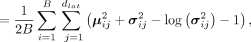
To integrate shared biological variation information in reference data, we assume elements in P are subject to a prior Gaussian distribution parameterized by μp and  , where μp is the PCA projection weight matrix of the reference gene expression matrix and σp contains elements equal to one-tenth standard deviation of μp. The step-by-step construction of reference gene expression matrix from various sources is illustrated in Supplemental Text S1 and Supplemental Algorithm S4. KLD is used to restrict the distance between the Gaussian distribution parameterized by the parameters of BNN module and
the prior Gaussian distribution parameterized by reference data:
, where μp is the PCA projection weight matrix of the reference gene expression matrix and σp contains elements equal to one-tenth standard deviation of μp. The step-by-step construction of reference gene expression matrix from various sources is illustrated in Supplemental Text S1 and Supplemental Algorithm S4. KLD is used to restrict the distance between the Gaussian distribution parameterized by the parameters of BNN module and
the prior Gaussian distribution parameterized by reference data:

Self-attention mechanism
Self-attention mechanism is the key mechanism of transformer for capturing the relationship between words in a given sentence in machine translation tasks, showing superior performance compared with other recurrent neural network-based models (Vaswani et al. 2017; Raffel et al. 2020). Recent advances have revealed that gene expression levels of neighboring spots in a tissue microenvironment tend to be correlated (Dries et al. 2021; Dong and Zhang 2022; Zeng et al. 2022). Inspired by the above understanding, PAST adopts a self-attention mechanism to model the relationship between neighboring spots (Fig. 1E).
The input of the self-attention module is a feature matrix M and the corresponding k-NN graph G. G is constructed using spatial coordinates with k = 6. The input matrix M is mapped to obtain query Q, key K, and value V through three FCNs, and the adjacent matrix A can then be calculated as follows: where dk is the feature dimension of query Q and key K. The attention weight matrix A can be obtained by normalizing the adjacent matrix A,
 where Aij is the attention weight from spot j to spot i, and Si denotes the set of neighbors of spot i in G. To avoid excessive spatial smoothing of hidden features, we add a shortcut in the self-attention module (Zhang and Meng 2019; Liu et al. 2021) and the output of self-attention module can be written as the subsequent form:
 where fattn( · ) denotes the function of self-attention module.
Loss function
Analysis of omics data is susceptible to sequencing noise such as dropout, and recent studies have proven that it is beneficial
to consider data sparsity and dropout in spatial transcriptomic data (Shengquan et al. 2021). Here we design sparsity adaptive reconstruction loss based on the insight that the higher the data sparsity, the more serious
the dropout phenomenon is, and the higher probability the zero gene expression observations are false negative. Given a minibatch
containing B spots and M genes, the sparsity adaptive reconstruction loss is shown as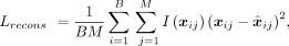 where xij denotes the profiled expression level of gene j in spot i,
  denotes the reconstructed expression level of gene j in spot i, and the function I( · ) is (si represents the sparsity of spot i)
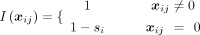 We assume the low-dimensional embeddings follow multivariate Gaussian distribution and the prior is the centered isotropic
multivariate Gaussian distribution. The distance between the latent distribution and the prior distribution is restricted
by KLD (Kingma and Welling 2014):
We assume the low-dimensional embeddings follow multivariate Gaussian distribution and the prior is the centered isotropic
multivariate Gaussian distribution. The distance between the latent distribution and the prior distribution is restricted
by KLD (Kingma and Welling 2014):
 where μ and σ are the mean vectors and standard deviation vectors of latent space, respectively, whereas dlat denotes the dimension of latent space.
Metric learning has been proposed to model the distance between samples, making the distance between positive sample pairs
closer and the distance between negative sample pairs farther (Hadsell et al. 2006). Samples in spatial transcriptomics are of strong spatial autocorrelation, which means that spatial neighboring spots may
have similar gene expression patterns and tend to belong to the same functional structure (Zeng et al. 2022). Here we design a metric learning loss function to restrict the distance of low-dimensional representations between neighbor
samples: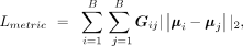 where G is the weighted spatial neighbor graph and the connection weights between samples are calculated using the Student's t-distribution kernel, μi and μj denote the latent embeddings of spot i and spot j, respectively. The calculation of G can be denoted as
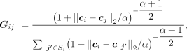 where ci denotes the spatial coordinate of spot i, Si denotes the set of neighbors of spot i, α is a scale factor that is set to 1 by default. We also tried to build the graph G with gene expression information of spots, that is, denoting the above ci as gene expression vector of spot i, and compared the two different approaches (Supplemental Text S12; Supplemental Fig. S33), illustrating the effectiveness of building graph G with spatial information.
As described in the above section, we integrate prior information through the BNN (Blundell et al. 2015) module and restrict the distance between parameter of the BNN module and prior distribution through Lbnn loss function. The objective function of PAST is the combination of the aforementioned four parts: where β1, β2, β3, β4 are coefficients served as a trade-off between the four parts and we set β1 = 1, β2 = 1, β3 = 1, β4 = 1 by default. We have evaluated the impact of the four coefficients and the contribution of the four loss function parts
through experimental analysis, which finally illustrates the robustness of PAST to different hyperparameter settings and the
significance of each part of the loss function (Supplemental Text S13; Supplemental Figs. S34, S35).
where β1, β2, β3, β4 are coefficients served as a trade-off between the four parts and we set β1 = 1, β2 = 1, β3 = 1, β4 = 1 by default. We have evaluated the impact of the four coefficients and the contribution of the four loss function parts
through experimental analysis, which finally illustrates the robustness of PAST to different hyperparameter settings and the
significance of each part of the loss function (Supplemental Text S13; Supplemental Figs. S34, S35).
Multislice joint embedding and automatic annotation
We propose two strategies, namely a transfer learning strategy and a 3D stacking strategy, to apply representation learning methods designed for single slice to multiple slices for joint embedding. Furthermore, we annotate the domain labels of multiple slices in ST data based on the joint embeddings obtained by the aforementioned strategies. The detailed explanations of the joint embedding and automatic annotation strategies are shown in Supplemental Text S4.
Baseline methods, downstream analyses, and evaluation metrics
Downstream applications including visualization, clustering, trajectory inference, and pseudotime analysis are detailed in Supplemental Text S3. To evaluate the performance of our model, we benchmarked PAST with nine baseline methods in term of 16 quantitative metrics and various downstream analyses. We describe the baseline methods, parameter settings, and the evaluation metrics in Supplemental Text S2. The details about data collection and preprocessing are shown in Supplemental Text S9. The information about all the target data sets and reference data sets is summarized in Supplemental Table S8.
Data sets
The STARmap mouse primary visual cortex (MPVC) data set (Wang et al. 2018) is available at https://kangaroo-goby.squarespace.com/data. The 10x Visium dorsolateral prefrontal cortex (DLPFC) data set (Maynard et al. 2021) includes 12 slices from 3 neurotypical adult donors and is accessible through http://spatial.libd.org/spatialLIBD. The osmFISH mouse somatosensory cortex (MSC) data set (Codeluppi et al. 2018) is available at website http://linnarssonlab.org/osmFISH/availability/. The Stereo-seq mouse olfactory bulb (Chen et al. 2022a) Sections 1 (MOBS1) and Section 2 (MOBS2) are accessible at https://db.cngb.org/stomics/mosta/download/, where MOBS2 was taken as the reference data for MOBS1. The 10x Visium human breast cancer Section 1 (BCS1) was precisely annotated by Fu et al. (2021), whereas Section 2 (BCS2) is not manually annotated, available at the 10x Genomics website https://www.10xgenomics.com/resources/datasets/human-breast-cancer-block-a-section-1-1-standard-1-1-0 and https://www.10xgenomics.com/resources/datasets/human-breast-cancer-block-a-section-2-1-standard-1-1-0, respectively. The three Stereo-seq axolotl brain data sets (Wei et al. 2022) identified by 2DPI are available through the website https://db.cngb.org/stomics/artista/download/. The Stereo-seq zebrafish embryo data set (Liu et al. 2022a) contains 12 slices of 12 h post-fertilization zebrafish embryo and can be downloaded from https://db.cngb.org/stomics/zesta/download/. The 10x Visium mouse brain coronal data set is accessible through https://support.10xgenomics.com/spatial-gene-expression/datasets/1.1.0/V1_Adult_Mouse_Brain. The Stereo-seq mouse brain data set (Chen et al. 2022a) can be downloaded from https://db.cngb.org/stomics/mosta/download. The scRNA-seq mouse primary visual cortex data set was obtained from the NCBI Gene Expression Omnibus (GEO; https://www.ncbi.nlm.nih.gov/geo/) under accession number GSE71585.
Software availability
The PAST algorithm is implemented in Python and the source code for reproduction is available at GitHub (https://github.com/lizhen18THU/PAST) and Supplemental Code. We also provided detailed documentation and step-by-step tutorials for applying PAST to ST data generated by different technologies at Read the Docs website (https://past.readthedocs.io/en/latest).
Competing interest statement
The authors declare no competing interests.
Acknowledgments
This work was supported by the National Key Research and Development Program of China Grant No. 2021YFF1200902 (R.J.), the National Natural Science Foundation of China Grants No. 62203236 (S.C.), No. 62273194 (R.J.), No. 61721003 (X.Z.), and the Fundamental Research Funds for the Central Universities, Nankai University, Grant No. 63231137 (S.C.).
Author contributions: S.C. conceived the study and supervised the project. Z.L. and S.C. designed, implemented, and validated PAST. X.C. and X.Z. helped with analyzing the results. S.C., Z.L., X.Z., and R.J. wrote the manuscript, with input from all the authors.
Footnotes
-
[Supplemental material is available for this article.]
-
Article published online before print. Article, supplemental material, and publication date are at https://www.genome.org/cgi/doi/10.1101/gr.277891.123.
-
Freely available online through the Genome Research Open Access option.
- Received March 16, 2023.
- Accepted September 19, 2023.
This article, published in Genome Research, is available under a Creative Commons License (Attribution-NonCommercial 4.0 International), as described at http://creativecommons.org/licenses/by-nc/4.0/.


