
Inferring gene expression from ribosomal promoter sequences, a crowdsourcing approach
- Pablo Meyer1,6,
- Geoffrey Siwo2,
- Danny Zeevi3,
- Eilon Sharon4,
- Raquel Norel1,
- DREAM6 Promoter Prediction Consortium5,
- Eran Segal4 and
- Gustavo Stolovitzky1
- 1IBM T.J. Watson Research Center, Yorktown Heights, New York 10598, USA;
- 2Eck Institute for Global Health, Department of Biological Sciences, University of Notre Dame, Notre Dame, Indiana 46556, USA;
- 3Lewis-Sigler Institute for Integrative Genomics, Princeton University, Princeton, New Jersey 08540, USA;
- 4Department of Computer Science and Applied Mathematics, Weizmann Institute of Science, Rehovot 76100, Israel
- 7Eck Institute for Global Health, Department of Biological Sciences, University of Notre Dame, Notre Dame, Indiana 46556, USA;
- 8Interdisciplinary Center for Network Science and Applications (iCeNSA), University of Notre Dame, Notre Dame, Indiana 46556, USA;
- 9Genome and Systems Biology Degree Program, National Taiwan University and Academia Sinica, Taipei 106, Taiwan;
- 10Department of Bio-Industrial Mechatronics Engineering, National Taiwan University, Taipei 106, Taiwan;
- 11Electrical Engineering Department, Texas A&M University, College Station, Texas 77843, USA;
- 12Swiss Institute for Experimental Cancer Research (ISREC), School of Life Sciences, Swiss Federal Institute of Technology (EPFL), CH-1015 Lausanne, Switzerland;
- 13Center for Genome Sciences and Systems Biology and Department of Computer Science, Washington University, St. Louis, Missouri 63110, USA;
- 14Laboratory of Immunoregulation and Mucosal Immunology, Department for Molecular Biomedical Research, VIB, Ghent University, 9052 Gent, Belgium;
- 15Department of Plant Systems Biology, VIB, Ghent University, 9052 Gent, Belgium;
- 16Department of Plant Biotechnology and Bioinformatics, Ghent University, 9052 Gent, Belgium;
- 17Max Planck Institute for Molecular Genetics, 14195 Berlin, Germany;
- 18Institute of Molecular Biology, 55128 Mainz, Germany;
- 19Institute for Medical Genetics, Universitätsklinikum Charité, 13353 Berlin, Germany;
- 20The Institute for Quantitative Biology, East Tennessee State University, Johnson City, Tennessee 37614-0663, USA;
- 21Interdisciplinary Centre for Mathematical and Computational Modeling, University of Warsaw, 00-927 Warsaw, Poland;
- 22School of Mathematics and Statistics, University of Hyderabad, Hyderabad-500046, India;
- 23Department of Mathematical Sciences, Department of Biology, Biocenter Oulu, University of Oulu, FIN-90014 Finland;
- 24Department of Mathematics, MIT, Cambridge, Massachusetts 02139, USA;
- 25Department of Microbial and Molecular Systems, KU Leuven, Leuven, Belgium;
- 26Department of Mathematics & Computer Sciences, University of Antwerp, B2020 Antwerp, Belgium;
- 27Biomedical Informatics Research Center Antwerp (biomina), University of Antwerp, B2020 Antwerp, Belgium;
- 28Fondazione Edmund Mach, Research and Innovation Centre, 38010 Trento, Italy;
- 29Department of Computer Science, Duke University, Durham, North Carolina 27708, USA;
- 30Department of Biostatistics and Computational Biology, Dana-Farber Cancer Institute, Department of Biostatistics, Harvard School of Public Health, Boston, Massachusetts 02115, USA
Abstract
The Gene Promoter Expression Prediction challenge consisted of predicting gene expression from promoter sequences in a previously unknown experimentally generated data set. The challenge was presented to the community in the framework of the sixth Dialogue for Reverse Engineering Assessments and Methods (DREAM6), a community effort to evaluate the status of systems biology modeling methodologies. Nucleotide-specific promoter activity was obtained by measuring fluorescence from promoter sequences fused upstream of a gene for yellow fluorescence protein and inserted in the same genomic site of yeast Saccharomyces cerevisiae. Twenty-one teams submitted results predicting the expression levels of 53 different promoters from yeast ribosomal protein genes. Analysis of participant predictions shows that accurate values for low-expressed and mutated promoters were difficult to obtain, although in the latter case, only when the mutation induced a large change in promoter activity compared to the wild-type sequence. As in previous DREAM challenges, we found that aggregation of participant predictions provided robust results, but did not fare better than the three best algorithms. Finally, this study not only provides a benchmark for the assessment of methods predicting activity of a specific set of promoters from their sequence, but it also shows that the top performing algorithm, which used machine-learning approaches, can be improved by the addition of biological features such as transcription factor binding sites.
One of the main objectives of the Dialogue for Reverse Engineering Assessments and Methods (DREAM) (Stolovitzky et al. 2007) is to catalyze the interaction between experiment and theory in systems biology, particularly for quantitative model building. For this purpose, unpublished data is used to objectively test team predictions generated by their methods/algorithms. The evaluation of participants’ methods is blind, as inspired by the community challenges posed in CASP (Critical Assessment of Techniques for Protein Structure Prediction). CASP’s main goal is to obtain an in-depth and objective assessment of state-of-the-art techniques for protein structure prediction using a set of unpublished protein structures (Moult et al. 1995; Shortle 1995; Moult 1996). This same principle is used in DREAM where a blind benchmark is provided so predictions from different algorithms can be easily compared, thus enhancing the reliability of programs/methods used. We describe here the Gene Promoter Expression Prediction challenge from DREAM6, identify the best performers, and discuss the main results, as well as an improvement of the top-performing algorithm. The full description of the challenge, as was presented to the participants, including the teams' rankings, can be found at the DREAM website (http://the-dream-project.org).
Gene Promoter Expression Prediction challenge
The level at which genes are transcribed is determined in large part by the DNA sequence upstream of the gene, known as the promoter region. Although widely studied, we are still far from a quantitative and predictive understanding of how transcriptional regulation is encoded in cis-regulatory elements of gene promoters (Kaplan et al. 2009; Sharon et al. 2012). One obstacle in the field is obtaining accurate measurements of transcription derived from different promoters. Fusion of promoters to fluorescent reporters can be used to determine the relative contribution of transcription to the resulting mRNA levels, since they provide measurements of promoter activity independent of the sequence of the associated transcript (Kalir et al. 2001). To further address this, an experimental system was designed to measure the transcription derived from different promoters, all of which are inserted into the same genomic location upstream of a reporter gene―a yellow fluorescence protein gene (YFP) (Zeevi et al. 2011).
To study a set of promoters that share many regulatory elements and thus are suitable for computational learning, data pertaining to promoters of most of the ribosomal protein (RP) genes in yeast Saccharomyces cerevisiae grown in a rich medium condition was obtained (Zeevi et al. 2011). Although ribosomal promoters may not capture generic promoter features, the challenge presented sought to model RP promoters to address questions left unanswered by successful genome-wide models (Beer and Tavazoie 2004; Gertz and Cohen 2009; Irie et al. 2011), such as what are the mechanisms behind the equimolar expression of the RP genes despite their varying copy numbers and how the information for fine-tuned expression is encoded in promoter regions. Also, understanding the basis of fine-tuned regulation of highly homologous promoters could provide clues to engineer promoter libraries of desired activity, starting from a parent promoter sequence.
The promoter regions for the S. cerevisiae RP genes were defined as the sequence immediately upstream of the ribosomal protein coding region beginning at the translation start site (TrSS) and continuing 1200 bp or until reaching another upstream gene’s coding sequence, selecting whichever came first. This removes a source of variability between strains derived from post-transcriptional regulation related to the coding and 3′ untranslated regions. Each promoter was linked to a URA3 selection marker (Linshiz et al. 2008) and inserted into the same fixed location in the yeast genome (Gietz and Schiestl 2007) of a master strain that contained the YFP gene (see Fig. 1A). In addition to 110 natural RP promoter strains, we constructed 33 strains with site-specific mutated RP promoters using similar methods (Gietz and Schiestl 2007; Linshiz et al. 2008).
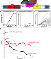
Overview of the experimental system and results. (A) Illustration of the master strain into which we integrated all the tested promoters. At a fixed chromosomal location, the master strain contains a gene that encodes a red fluorescent protein (mCherry), followed by the promoter for TEF2, and a gene that encodes for a yellow fluorescent protein (YFP). Every tested promoter is integrated into this strain, together with a selection marker, between the TEF2 promoter and the YFP gene. (B) Strains with different promoters have highly similar growth rates. Shown is the growth of 71 different promoter strains, measured as optical density (OD). Measurements were obtained from a single 96-well plate, with glucose-rich media and a small number of cells from each strain inserted into each well at time zero. The exponential growth phase is indicated (vertical dashed gray lines). (C) Same as B, but where the measurements correspond to mCherry intensity. Note the small variability in the intensity of mCherry, which is driven by the same control promoter across the different strains. (D) Same as C, but where the measurements correspond to YFP intensity. Note the large variability in the intensity of YFP, which is driven by a different promoter in each strain. (Adapted with permission from Zeevi et al. [2011].) (E) Black line shows the scores from different participating teams plotted in descending order, and red line shows scores of aggregated teams starting with the score obtained from averaging the prediction results of the two best-performing teams, followed by the three best-performing teams, and so on until all 21 teams are included. The stand-alone dot represents the post-hoc model combining SVM and biological features.
The strains containing the different RP derived promoters were synchronized and grown, and their YFP fluorescence was recorded in a plate reader. The transcription initiated by each promoter was measured by its promoter activity, defined as the average YFP fluorescence during the exponential growth phase divided by the average optical density (OD) during that time period (see Fig. 1B,D). Hence, promoter activity represents the average rate of YFP production from each promoter, per cell per second, during the exponential phase of growth (Zeevi et al. 2011). As a control for the experimental error, a red fluorescent protein (mCherry) was driven by a control promoter, identical in all strains (see Fig. 1C). Several tests were performed to gauge the accuracy and sensitivity of the system. The results showed that growth curves of all strains were nearly identical, YFP levels of independent clones of the same promoter sequence were indistinguishable from those of replicate measurements of the same clone, signals measured in the YFP wavelength were not affected by the presence of the mCherry protein, and no correlation was found between the YFP and mCherry promoter activities across the different RP promoter strains. Finally, the average difference between any two mCherry strains was ∼5%, and when using replicate measurements, the relative error in the estimated YFP promoter activity of an RP promoter is ∼2%, indicating that it is possible to distinguish between any two promoters whose activities differ by as little as ∼8% (Zeevi et al. 2011).
The challenge
The challenge consisted of predicting the promoter activity derived from a given RP promoter sequence. Participants were provided with a training set of 90 natural RP promoters (see Supplemental Table S1) for which both the promoter sequence and activity were known and a test set of 53 promoters (see Supplemental Table S2) for which only the promoter sequence was given. The test set was divided into two subsets. The first subset had 20 natural RP promoters. The second subset contained 33 promoters that are similar to natural RP promoters but have some mutations in their sequence. These mutations can be separated into six types: mutations of TATA boxes (Basehoar et al. 2004), of binding sites for Fhl1 and Sfp1―known transcriptional regulators of RP genes (Badis et al. 2008; Zhu et al. 2009), mutations to nucleosome disfavoring sequences, random mutations that occurred unintentionally while creating the natural promoters, and finally, sequences mutated intentionally with additional random mutations (see Table 1). The goal was to predict as accurately as possible the promoter activity of the 53 promoters in the test set using the 90 promoters for training.
Information on the promoter sequence mutations
Results and analysis
The challenge was scored in four different ways using criteria that considered the “distance” between measured and predicted values or differences in rank between measured and predicted values. The first metric consists of a Pearson correlation between the predicted and measured promoter activity. The second metric is a normalized sum of squared differences. The third is the Spearman rank correlation, which is essentially the Pearson correlation between the ranks, and the fourth metric is a normalized sum of the squared difference in ranks. These metrics were then combined into a score (see Methods, Eqs. 1–5).
As shown in Figure 1E and Table 2, out of 21 participating teams, team FiRST was the best performer, with a score of 1.88, followed by team c4lab with 1.55, in a close race for the second place with the third team, which was then followed by a monotonous decrease in the participants’ scores. When a series of aggregated teams are formed by averaging the predicted promoter activity values of the best N teams, the score of the aggregated best 15 teams becomes 1.49, close to that of the second-best performing team (c4lab) (see Fig. 1E). Scores for the remaining aggregated teams are also observed to be above the fourth ranked team, showing that blending community predictions produces robust results (see Supplemental Material, DREAM6 Participants Predictions files).
Scores from different teams ranked in descending order
We analyzed whether some participants were better at predicting specific promoters but could not find any correlation between overall team ranking and the number of promoters a team predicted best. Also, when predicting single promoters, the overall highly ranked methods did not rank first more often than lower ranked ones but fared well across all promoters.
In order to investigate whether some promoters were harder to predict, we calculated the average distance  over all participants for promoter i from the promoter’s predicted value to its measured value (see Eq. 6, Methods). As seen in Figure 2A, where promoters are ordered by increasing
  , five promoters out of the 53 stand out for being predicted with less accuracy. We next divided the promoters based on
  into two groups consisting of the best 30 predictions (green dots, Fig. 2A) and the 23 worst predictions (red dots, Fig. 2A) and plotted the Pearson correlation of each of the participating teams for these two groups of promoters (Fig. 2B). For all teams, the Pearson correlation clearly separated the best-predicted and worst-predicted promoters as defined by
 , showing that, for all participants, promoters could be consistently divided into two groups, one of which was harder to
predict than the other.
, showing that, for all participants, promoters could be consistently divided into two groups, one of which was harder to
predict than the other.
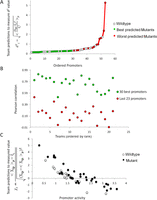
Analysis of promoter prediction results. (A) Promoters are ordered by increasing  , where
  is the predicted value of promoter i and participant p = 1,2…21 , and
  is the measured value for promoter i = 1,2…53. Green dots represent the 30 best predictions, and red dots the 23 worst predictions. Empty dots represent the 20
wild-type promoters; full dots represent the 33 mutated promoters. (B) The Pearson correlation of each of the participating teams is shown in green dots for the best predictions and in red dots
for the worst predictions as defined in A. Teams are ordered by rank based on their final score. (C) For each promoter, χi is plotted in logarithmic scale against the promoter activity value. Empty dots represent wild-type promoters and full dots
mutant promoters.
is the measured value for promoter i = 1,2…53. Green dots represent the 30 best predictions, and red dots the 23 worst predictions. Empty dots represent the 20
wild-type promoters; full dots represent the 33 mutated promoters. (B) The Pearson correlation of each of the participating teams is shown in green dots for the best predictions and in red dots
for the worst predictions as defined in A. Teams are ordered by rank based on their final score. (C) For each promoter, χi is plotted in logarithmic scale against the promoter activity value. Empty dots represent wild-type promoters and full dots
mutant promoters.
To identify the source of the difficulty in predicting the expression values of these 23 promoters, we explored the possibility
of this list being enriched for mutant promoters. Wild-type promoters were found to be distributed equally between the worst-predicted
promoters (10 empty dots on red side of Fig. 2A) and best-predicted promoters (10 empty dots on green side of Fig. 2A). A Fisher test shows no statistical significance for mutant or wild-type promoter enrichment. We next used measure  (see Eq. 7, Methods) to evaluate whether promoter activity was correlated to the difficulty of predicting its value. Figure 2C, showing how
  varies for each promoter, reflects that participants’ performance is anti-correlated with promoter activity, with a Pearson
correlation of −0.836. Participants’ prediction accuracy can be divided into three groups according to their promoter activity
varies for each promoter, reflects that participants’ performance is anti-correlated with promoter activity, with a Pearson
correlation of −0.836. Participants’ prediction accuracy can be divided into three groups according to their promoter activity
 :
:  values between 1 and 3 (
 0.25 ± 0.73 for
  such that 1 >
  > 3, 18 promoters)―which fared significantly better than the following two groups:
  values less than 1 (
 3.02 ± 1.10 for
  such that
  < 1, 8 promoters, t-test p < 1.1 × 10⁻¹¹); and
  values higher than 3 (
 −1.48 ± 0.51 for
  such that
  > 3, 7 promoters, t-test p < 1.75 × 10⁻⁷). Both observations are independent of whether the promoters contain mutations (Fig. 2C, full and empty dots).
As we could not find clear differences between mutant and wild-type promoters when using the  measure, we calculated a different type of distance
  to compare participant predictions and measurements (see Eq. 8, Methods). As shown in Figure 3A,
  clearly distinguishes wild-type promoters (mean value of
  is 1.62 ± 0.22) from mutant promoters (mean value of
  is 2.23 ± 0.41, t-test P < 8 × 10⁻⁸). In order to understand the differences in
  for the various mutant promoters, we formed six groups according to the nature of their mutations. In Figure 3B, the different groups of mutations were ordered according to the associated
  mean value. Participants’ predictions fared better for mutations typically inducing small changes in promoter expression
(low
mean value. Participants’ predictions fared better for mutations typically inducing small changes in promoter expression
(low  in Fig. 3B), such as random mutations. Conversely, sequence mutations known to induce large changes by lowering promoter expression,
such as mutations to the TATA box, were the worst-predicted group (high
in Fig. 3B), such as random mutations. Conversely, sequence mutations known to induce large changes by lowering promoter expression,
such as mutations to the TATA box, were the worst-predicted group (high  in Fig. 3B). As there is not enough data to extract a statistical measure of the differences between groups of promoters, we decided
to follow up on the previous observation and compare the
in Fig. 3B). As there is not enough data to extract a statistical measure of the differences between groups of promoters, we decided
to follow up on the previous observation and compare the  value for each mutant promoter to the relative promoter activity difference induced by the mutations. As shown in Figure 3C,
  grows exponentially with increasing differences between wild-type and mutant promoter expression. Hence, prediction accuracy
for mutant promoters worsened when mutations induced higher changes on expression.
grows exponentially with increasing differences between wild-type and mutant promoter expression. Hence, prediction accuracy
for mutant promoters worsened when mutations induced higher changes on expression.
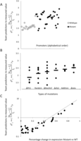
Analysis of prediction results for mutated promoters. (A) Promoters were divided into two groups depending on whether they were wild type (empty dots) or contained mutations (full
dots) and plotted according to  , where
  is the predicted value of promoter i and participant p = 1,2…21, and
  is the measured value for promoter i = 1,2…53. (B) Mutant promoter expression values were grouped according to the nature of the mutation and ordered by mean
  value for each group. The six groups consist of mutations of TATA boxes (Δtata), of binding sites for Fhl1 (Δfhl1) and Sfp1
(Δsfp1), mutations to nucleosome disfavoring sequences (ΔNucDisf), random mutations (Random), and finally, sequences mutated
intentionally with additional random mutations (Addition). The
value for each group. The six groups consist of mutations of TATA boxes (Δtata), of binding sites for Fhl1 (Δfhl1) and Sfp1
(Δsfp1), mutations to nucleosome disfavoring sequences (ΔNucDisf), random mutations (Random), and finally, sequences mutated
intentionally with additional random mutations (Addition). The  value for each promoter is indicated by full dots; the mean value of
  for each of the six grouped mutations is indicated by a thick bar. (C) For each mutated promoter i,
  is plotted as a function of the percentage of expression value change induced in the wild-type promoter by the mutation.
The vertical scale is logarithmic.
is plotted as a function of the percentage of expression value change induced in the wild-type promoter by the mutation.
The vertical scale is logarithmic.
Improving promoter expression prediction by adding biological features
As shown in Figure 1B, scores of aggregated teams were observed to be robustly above the fourth-ranked team but did not fare better than the three
best-performing teams. As the best-performing models of this challenge did not include biological features such as the binding
sites for Fhl1 and Sfp1, known transcriptional regulators of RP transcription factors, we decided to try to improve model
performance by including biological features in the best-performer algorithm of team FiRST. To do this, we modified a recently
published mechanistically motivated model that takes into account the competition between transcription factors and nucleosomes
for DNA binding sites in the regulation of gene expression (Zeevi et al. 2011) (Eqs. 9 and 10; see Methods). The score for this model based on  , the Pearson correlation between predicted and observed activity, was 0.49 (see Eq. 1, Methods). We then combined this model
with that of the best-performing team, FiRST, in two ways. In the first approach, we averaged the predicted activity of each
promoter by team FiRST and the mechanistic model. The correlation between the predicted and actual activities remained the
same as for FiRST (∼0.65) (see Table 1), demonstrating the robustness of aggregating predictions even when one method has considerably lower performance. Given
that the method by team FiRST did not explicitly use transcription factor binding, we reasoned that incorporating the transcription
factor binding site information directly into team FiRST’s model should be complementary to the method and could reveal interactions
between transcription factors and sequence context. To test this idea, we included the transcription factor binding affinities
for each promoter as additional features to those used by team FiRST (see Supplemental Table S3 for details on the features).
We then trained a support vector machine (SVM) using the combined features from both models. The resulting model provided
predictions that had a correlation of 0.67 to the actual promoter activity and a combined score of 2.6 (Cp = 0.67289; X2 = 39.79601; Sp = 0.66815; R2 = 30.75429) (see Fig. 1E and Supplemental Data, DREAM6 Participants Predictions files), presenting a significant improvement and best performance
compared to all the other teams or the aggregate of their predictions.
, the Pearson correlation between predicted and observed activity, was 0.49 (see Eq. 1, Methods). We then combined this model
with that of the best-performing team, FiRST, in two ways. In the first approach, we averaged the predicted activity of each
promoter by team FiRST and the mechanistic model. The correlation between the predicted and actual activities remained the
same as for FiRST (∼0.65) (see Table 1), demonstrating the robustness of aggregating predictions even when one method has considerably lower performance. Given
that the method by team FiRST did not explicitly use transcription factor binding, we reasoned that incorporating the transcription
factor binding site information directly into team FiRST’s model should be complementary to the method and could reveal interactions
between transcription factors and sequence context. To test this idea, we included the transcription factor binding affinities
for each promoter as additional features to those used by team FiRST (see Supplemental Table S3 for details on the features).
We then trained a support vector machine (SVM) using the combined features from both models. The resulting model provided
predictions that had a correlation of 0.67 to the actual promoter activity and a combined score of 2.6 (Cp = 0.67289; X2 = 39.79601; Sp = 0.66815; R2 = 30.75429) (see Fig. 1E and Supplemental Data, DREAM6 Participants Predictions files), presenting a significant improvement and best performance
compared to all the other teams or the aggregate of their predictions.
Discussion
The scoring and analysis of submitted predictions for the DREAM6 Gene Promoter Expression Prediction challenge revealed excellent performances (see Fig. 1E and Table 2). This is, indeed, remarkable, as the data set presented a difficult learning problem due to the high homology between the promoters in the relatively small RP promoter training set―yeast only has 137 ribosomal promoters―and lower dynamic range of promoter activity compared to what would be observed on a genome-wide scale. Methods with typically high accuracy in genome-wide predictions ranked 11 and 12 here (see Supplemental Table S4), indicating that the challenge posed by RP promoters is distinct and requires the development of specific methods in order to be solved.
Choosing the right scoring scheme to evaluate the challenge was essential, as participants fared differently depending on the metric used (see Table 2). The best-performing team did not get the top score for all metrics nor all promoters but was the most consistent. Also, participants had difficulties while predicting low-expressed promoters and certain mutant RP promoters. Finally, community predictions were robust to the aggregation of teams’ results, and the best score of 2.6 was obtained by combining features from team FiRST’s machine-learning model and a mechanistic model based on biophysical assumptions.
During their presentations at the DREAM6 conference, the best-performing teams, FiRST and c4lab, showed that mutated promoters were harder to predict than natural promoters. Team FiRST mainly used the first 100 bp of the promoter to predict promoter activity, and team c4lab used a 12-mer motif. Team FiRST tried to include features such as k-mer counts (mono, di, tri, tetra, and penta), homopolymer stretches, promoter length, DNA bendability, DNA protein deformability, DNA bending stiffness, and nucleosome binding potential. They used a machine-learning SVM approach to select 12 features that can be summarized as follows: one mononucleotide G, one dinucleotide GT, six trinucleotides, 12 tetranucleotides, length of T-tracts and TA-tracts, DNA deformability (a detailed description of this model will appear in a different manuscript). Team c4lab also used different k-mer counts to finally concentrate on 12-mer motifs used in a support vector regression approach but did not find any correlation between the 12-mers and biological features such as distance to a TrSS or copy number motifs (see Supplemental Table S4 for a brief description of other participants’ methods).
Neither of the best-performing teams directly used general features related to transcription factors such as TATA boxes and nucleosome occluding sequences. Actually, none of the four biological features targeted by the mutations―TATA boxes, binding sites for the transcriptional regulators Fhl1 and Sfp1, and mutations to nucleosome disfavoring sequences―were detected by the participants. Since most participants did not include these features in their models, it is not surprising that many fared worse with promoters where these sequences were mutated. Figure 3, B and C show precisely that, as mutation-induced expression changes increase, predictions become worse. One exception is team FiRST’s machine-learning method that was able to identify a number of nucleosome disfavoring features, in particular TA-tracts, as being useful in predicting promoter activity.
During the DREAM6 conference discussion, an audience member proposed that the training set should have included mutated promoter sequences. However, an intended feature of the challenge was to indicate that mutated sequences were present in the test set without giving hints or providing training data on sequence changes that could affect the promoter expression level. We expected participants to analyze the origin of these mutations and think that our strategy was correct, as Figure 2A shows that, although participants did not look for the origin of mutated promoters, these were distributed equally between the groups of best- and worst-predicted promoters. It is only when all mutated and wild-type promoters are separated into two groups that participants’ predictions for those two groups can be differentiated (Fig. 3A).
The mechanism by which Fhl1, Sfp1, Rap1, and TATA boxes contribute to the promoter expression appear to follow a simple rule, where more sites from these factors in closer proximity to the TrSS result in higher promoter activity (Zeevi et al. 2011). The contribution of one of these factors to the overall promoter activity depends on the specific organization of its sites within the promoter (Lieb et al. 2001; Wade et al. 2004; Sharon et al. 2012). As shown in Figure 2C, participants had difficulties predicting low- and high-expressed promoters. The thresholds for low/high promoter activity are sharply defined and define values lower than 1.5 and higher than 3, respectively. Seven of the eight promoters whose activity is higher than 3 are mutated promoters, shown to be difficult to predict. Low-activity promoters are RPL41B_Mut1, RPL15A_Mut1, RPL21B, RPL4A_Mut6, RPL11A, RPL35B, RPL39_Mut1, and RPS14B_Mut1. As the experimental setup can distinguish promoter activities separated by less than 8%, we do not think that the difficulties with predicting low promoters arise from experimental limitations while measuring lower signals. Instead, as shown in Table 1, promoters RPL41B_Mut1, RPL21B, RPL11A, RPL35B, RPL39_Mut1, and RPS14B_Mut1 have dispersed or lack binding motifs (see also Supplemental Table S5). The other mutations present in promoters of low activity are RPL4A_Mut6 and RPL15A_Mut1, which cause an ∼70% decrease in promoter activity, and as discussed, participants had difficulties predicting strong mutation effects. We conclude that the difficulty participants had while predicting low-expressed promoters is, indeed, due to less information available in these promoter sequences and a less coherent organization of the different sequence features, with very few TATA boxes, Fhl1, Rap1, and Sfp1 sites.
Finally, the improvement of the best-performing model, by mixing a biology-based mechanistic approach and machine-learning techniques, implies that the wisdom of crowds could be tapped further by methods that directly incorporate distinct features from independent models. Simple aggregation might miss the interactions between the different features in the models selected. Estimating the relative contributions of features extracted from each model could be approached as a learning problem where the different models are reduced to being independent tools for feature selection. Once the relevant features are selected, they are integrated into a new model, and adequate parameters are learned once again. Overall, we think this study not only provides a benchmark for the assessment of methods predicting promoter activity from sequence, but it also shows that understanding the basis of fine-tuned regulation of highly homologous promoters could provide clues for engineering promoter libraries to obtain a desired promoter strength from a parent promoter sequence.
Methods
Constructing promoter strains
A construct of ADH1 terminator–mCherry–TEF2 promoter–YFP– ADH1 terminator–NAT1 was inserted into the SGA-compatible strain Y8205 at the his3 deletion location (the construct replaced chromosome 15, at base pairs 721987–722506). The resulting strain served as a master strain for the entire library. Desired promoters were lifted by PCR from the BY4741 yeast strain. Primers contained one part matching the ends of the lifted promoters, and a constant part at their 5′ end matching the first 25 bases of the YFP gene (for reverse primers) or a linker sequence (for forward primers; see all primer sequences in Zeevi et al. 2011). Each promoter was linked to a URA3 selection marker (Linshiz et al. 2008) and then amplified such that its genomic integration sites increased to 45/50 bp. Integration into the genome was performed by homologous recombination as described in Gietz and Schiestl (2007). All steps were performed on 96-well plates, except for growing the final clones, which was performed on six-well plates (2% agar, SCD–URA). To validate the inserted promoter sequences, the insertions were lifted from each target strain by PCR and sequenced.
Constructing promoter strains with targeted mutations
To create a mutated promoter, we amplified it in two parts which flank the desired mutation area. The left part was amplified using a reverse primer with a 35-bp tail at its 5′ end that contains the desired mutation, while the right part was amplified using a forward primer that also had a similar tail. The two new parts, both containing the desired mutation in an overlapping region of 35 bp, were then connected, similar to the way in which we connected promoters to the URA3 selection marker. See Table 1 and Supplemental Table S6 for more information.
Library measurements
Cells were inoculated from stocks kept at −80°C into SCD (180 μL, 96-well plate) and left to grow at 30°C for 48 h, reaching complete saturation. Next, 8 μL were passed into fresh medium (180 μL) according to the desired condition (e.g., SCD, ethanol, heat shock). Measurements were carried out every ∼20 min using a robotic system (Tecan Freedom EVO) with a plate reader (Tecan Infinite F500). Each measurement included optical density (filter wavelengths 600 nm, bandwidth 10 nm), YFP fluorescence (excitation 500 nm, emission 540 nm, bandwidths 25/25 nm, accordingly), and mCherry fluorescence (excitation 570 nm, emission 630 nm, bandwidths 25/35 nm, accordingly). Measurements were carried out using a total of eight different conditions. In all experiments, yeast cells were grown on SC (6.9 g/L YNB, 1.6 g/L amino acids complete). Four conditions used different 2% sugar growth media: SC-glucose, SC-galactose, SC-ethanol, and SC-glycerol. The other four conditions used SC-glucose with an additional stress factor: Rapamycin (40 μg/mL), amino acid starvation (no amino acids except histidine and leucine), heat shock (39°C), and osmotic stress (750 mM KCl). Every strain was measured in three biological replicates for each condition. Most of the data analysis was performed on data from growth on SC-glucose (without stress), which was measured in five replicates.
Scoring
The challenge was scored in four different ways using criteria based on the “distance” between measured and predicted values
or differences in rank between measured and predicted values. As we requested predictions of the expression levels from N = 53 promoter sequences, let us denote by Xip the predicted activity of promoter i for participant p, and ξi the measured activity of promoter i = 1, 2 …, 53 and p = 1,2….,P, where P = 21 is the number of teams that participated in the challenge. The score based on a Pearson metric for participant p is
defined by
In order to calculate for each participant the probability of getting by chance a score at least as good, we randomly sampled
the predictions across the entire set of participants. For each promoter i = 1,2…53, we chose at random one of the  predictions, where p = 1,2,…,P. We thus obtained a value of
  which corresponded to one possible random choice of predictions among all the participants. By repeating the same process
100,000 times, we generated a null distribution of distances between measured and estimated values, from which a P-value can be estimated for
which corresponded to one possible random choice of predictions among all the participants. By repeating the same process
100,000 times, we generated a null distribution of distances between measured and estimated values, from which a P-value can be estimated for  . For each participant, that P-value was denoted as
  .
.
The score based on the χ2 metric for participant p is defined by
The null hypothesis was generated in a similar way by generating P-values resulting from the permutation of participants’ predicted values for a given promoter, and also for each participant,
and that P-value was denoted as  .
.
We also defined the score by comparing the rank of predicted values to the actual rank of measured values. Let us denote by
Rip the predicted rank of promoter i for participant p, 1< Rip <53 and ρi the rank of the measured promoter i = 1, 2 …, 53 and p = 1,2,…,P. Then, the score based on a Spearman metric for participant p is defined by
A null prediction was created by randomly permuting participants’ predicted values for a given promoter and then ranking a
given “random” participant i to obtain the Rip ranks across the 53 different rankings of promoters, thus generating a distribution of distances between measured and estimated
values, for which a P-value denoted as  can be estimated for
  . The score based on a rank2 metric for participant p is defined by
 where
where  is the rank of proximity of
  , 1 <
, 1 <  < P, and ρi the rank of the measured promoter i = 1, 2 …, 53. The null hypothesis was derived from the random permutation of participants’ predicted values for a given promoter
and then ranking a given “random” participant. The derived P-value is denoted as
< P, and ρi the rank of the measured promoter i = 1, 2 …, 53. The null hypothesis was derived from the random permutation of participants’ predicted values for a given promoter
and then ranking a given “random” participant. The derived P-value is denoted as  . The overall score was defined as a function of the product of all the P-values defined as
Prediction distances to promoter values
The average distance  over all participants p for promoter i from the promoter predicted value (
 ) to the promoter measured value (
 ) is defined as
We also considered whether promoter activity was correlated to the difficulty to predict its value and used the following
measure  defined by
We finally calculated a different type of distance  to compare participant predictions and measurements, defined such that
Combined model
We considered binding sites for three transcription factors―Rap1 (Wade et al. 2004), Fhl1 (Harbison et al. 2004; Schawalder et al. 2004; Wade et al. 2004), Sfp1 (Badis et al. 2008; Zhu et al. 2009)―that have been shown to influence yeast ribosomal gene expression. Our model considered promoter activity Xp as directly proportional to the binding likelihood of each of the three transcription factors to their cognate motifs, above
a specific threshold, relative to the nucleosome binding potential of the same sites: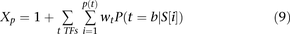 where P(t) is the set of all potential binding sites for transcription factor t above a certain threshold, wt is a coefficient measuring the relative contribution of factor t to the promoter activity determined using MATLAB’s nonlinear solver, and
  is the probability that transcription factor t binds its potential site at position i in promoter sequence S. To determine the binding sites for the three transcription factors, we used their sequence specificities documented in position
weight matrices (PWMs) (Basehoar et al. 2004; Badis et al. 2008; Zhu et al. 2009). In estimating the binding threshold for each transcription factor, we explored the correlation between promoter activity
and sites above each possible threshold at intervals of 0.1. For each transcription factor, we considered potential binding
sites as those with an affinity above the threshold and located within known spatial localization sites: for Rap1, 400 bp
upstream of the TrSS; for Fhl1 and Sfp1, 300 bp upstream of the TrSS (Zeevi et al. 2011). We then modeled the probability for transcription factor binding as the weight of the configuration in which the factor
is bound divided by the sum of the weight of that configuration, the weight of the configuration in which the DNA is unbound,
and the weight of the configuration in which a nucleosome is bound to the site:
is the probability that transcription factor t binds its potential site at position i in promoter sequence S. To determine the binding sites for the three transcription factors, we used their sequence specificities documented in position
weight matrices (PWMs) (Basehoar et al. 2004; Badis et al. 2008; Zhu et al. 2009). In estimating the binding threshold for each transcription factor, we explored the correlation between promoter activity
and sites above each possible threshold at intervals of 0.1. For each transcription factor, we considered potential binding
sites as those with an affinity above the threshold and located within known spatial localization sites: for Rap1, 400 bp
upstream of the TrSS; for Fhl1 and Sfp1, 300 bp upstream of the TrSS (Zeevi et al. 2011). We then modeled the probability for transcription factor binding as the weight of the configuration in which the factor
is bound divided by the sum of the weight of that configuration, the weight of the configuration in which the DNA is unbound,
and the weight of the configuration in which a nucleosome is bound to the site: where 1 represents the DNA unbound configuration,
  represents the affinity of transcription factor t for the binding site at position i in promoter S, and
  is the affinity of nucleosomes for position i in promoter S.
For  , we used a sequence-based nucleosome affinity model to compute the average nucleosome occupancy (Kaplan et al. 2009).
We applied wt coefficients obtained from a nonlinear solver trained on 90 promoters to predict promoter activities of a held-out set of 53 promoters used in the DREAM challenge.
DREAM6 consortium
Geoffrey Siwo,7 Andrew K. Rider,8 Asako Tan,7 Richard S. Pinapati,7 Scott Emrich,8 Nitesh Chawla,8 Michael T. Ferdig,7,8 Yi-An Tung,9 Yong-Syuan Chen,10 Mei-Ju May Chen,9 Chien-Yu Chen,9,10 Jason M. Knight,11 Sayed Mohammad Ebrahim Sahraeian,11 Mohammad Shahrokh Esfahani,11 Rene Dreos,12 Philipp Bucher,12 Ezekiel Maier,13 Yvan Saeys,14,15,16 Ewa Szczurek,17 Alena Myšičková,17 Martin Vingron,17 Holger Klein,18 Szymon M. Kiełbasa,17,19 Jeff Knisley,20 Jeff Bonnell,20 Debra Knisley,20 Miron B. Kursa,21 Witold R. Rudnicki,21 Madhuchhanda Bhattacharjee,22 Mikko J. Sillanpää,23 James Yeung,24 Pieter Meysman,25,26,27 Aminael Sánchez Rodríguez,25 Kristof Engelen,25,28 Kathleen Marchal,15,25 Yezhou Huang,29 Fantine Mordelet,29 Alexander Hartemink,29 Luca Pinello,30 and Guo-Cheng Yuan30
Acknowledgments
We thank Noam Kaplan from the Weizmann Institute of Science for computing the average nucleosome occupancies and Kahn Rhrissorrakrai for useful comments on the manuscript.
Footnotes
-
↵5 A complete list of consortium authors appears at the end of this manuscript.
-
↵6 Corresponding author
E-mail pmeyerr{at}us.ibm.com
-
↵7 Eck Institute for Global Health, Department of Biological Sciences, University of Notre Dame, Notre Dame, Indiana 46556, USA
-
↵8 Interdisciplinary Center for Network Science and Applications (iCeNSA), University of Notre Dame, Notre Dame, Indiana 46556, USA
-
↵9 Genome and Systems Biology Degree Program, National Taiwan University and Academia Sinica, Taipei 106, Taiwan
-
↵10 Department of Bio-Industrial Mechatronics Engineering, National Taiwan University, Taipei 106, Taiwan
-
↵11 Electrical Engineering Department, Texas A&M University, College Station, Texas 77843, USA
-
↵12 Swiss Institute for Experimental Cancer Research (ISREC), School of Life Sciences, Swiss Federal Institute of Technology (EPFL), CH-1015 Lausanne, Switzerland
-
↵13 Center for Genome Sciences and Systems Biology and Department of Computer Science, Washington University, St. Louis, Missouri 63110, USA
-
↵14 Laboratory of Immunoregulation and Mucosal Immunology, Department for Molecular Biomedical Research, VIB, Ghent University, 9052 Gent, Belgium
-
↵15 Department of Plant Systems Biology, VIB, Ghent University, 9052 Gent, Belgium
-
↵16 Department of Plant Biotechnology and Bioinformatics, Ghent University, 9052 Gent, Belgium
-
↵17 Max Planck Institute for Molecular Genetics, 14195 Berlin, Germany
-
↵18 Institute of Molecular Biology, 55128 Mainz, Germany
-
↵19 Institute for Medical Genetics, Universitätsklinikum Charité, 13353 Berlin, Germany
-
↵20 The Institute for Quantitative Biology, East Tennessee State University, Johnson City, Tennessee 37614-0663, USA
-
↵21 Interdisciplinary Centre for Mathematical and Computational Modeling, University of Warsaw, 00-927 Warsaw, Poland
-
↵22 School of Mathematics and Statistics, University of Hyderabad, Hyderabad-500046, India
-
↵23 Department of Mathematical Sciences, Department of Biology, Biocenter Oulu, University of Oulu, FIN-90014 Finland
-
↵24 Department of Mathematics, MIT, Cambridge, Massachusetts 02139, USA
-
↵25 Department of Microbial and Molecular Systems, KU Leuven, Leuven, Belgium
-
↵26 Department of Mathematics & Computer Sciences, University of Antwerp, B2020 Antwerp, Belgium
-
↵27 Biomedical Informatics Research Center Antwerp (biomina), University of Antwerp, B2020 Antwerp, Belgium
-
↵28 Fondazione Edmund Mach, Research and Innovation Centre, 38010 Trento, Italy
-
↵29 Department of Computer Science, Duke University, Durham, North Carolina 27708, USA
-
↵30 Department of Biostatistics and Computational Biology, Dana-Farber Cancer Institute, Department of Biostatistics, Harvard School of Public Health, Boston, Massachusetts 02115, USA
-
[Supplemental material is available for this article.]
-
Article published online before print. Article, supplemental material, and publication date are at http://www.genome.org/cgi/doi/10.1101/gr.157420.113.
- Received March 12, 2013.
- Accepted August 14, 2013.
This article is distributed exclusively by Cold Spring Harbor Laboratory Press for the first six months after the full-issue publication date (see http://genome.cshlp.org/site/misc/terms.xhtml). After six months, it is available under a Creative Commons License (Attribution-NonCommercial 3.0 Unported), as described at http://creativecommons.org/licenses/by-nc/3.0/.


