Haplotype-aware sequence alignment to pangenome graphs

Ghanshyam Chandra; Daniel Gibney; Chirag Jain

doi:10.1101/gr.279143.124

Abstract

Modern pangenome graphs are built using haplotype-resolved genome assemblies. When mapping reads to a pangenome graph, prioritizing alignments that are consistent with the known haplotypes improves genotyping accuracy. However, the existing rigorous formulations for colinear chaining and alignment problems do not consider the haplotype paths in a pangenome graph. This often leads to spurious read alignments to those paths that are unlikely recombinations of the known haplotypes. In this paper, we develop novel formulations and algorithms for sequence-to-graph alignment and chaining problems. Inspired by the genotype imputation models, we assume that a query sequence is an imperfect mosaic of reference haplotypes. Accordingly, we introduce a recombination penalty in the scoring functions for each haplotype switch. First, we solve haplotype-aware sequence-to-graph alignment in $O (| Q | | E | | H |)$ time, where Q is the query sequence, E is the set of edges, and H is the set of haplotypes represented in the graph. To complement our solution, we prove that an algorithm significantly faster than $O (| Q | | E | | H |)$ is impossible under the strong exponential time hypothesis (SETH). Second, we propose a haplotype-aware chaining algorithm that runs in $O (| H | N \log | H | N)$ time after graph preprocessing, where N is the count of input anchors. We then establish that a chaining algorithm significantly faster than $O (| H | N)$ is impossible under SETH. As a proof-of-concept, we implemented our chaining algorithm in the Minichain aligner. By aligning sequences sampled from the human major histocompatibility complex (MHC) to a pangenome graph of 60 MHC haplotypes, we demonstrate that our algorithm achieves better consistency with ground-truth recombinations compared with a haplotype-agnostic algorithm.

Pangenome graphs represent the maximum possible diversity that exists in the population (Singh et al. 2022). A variety of methods have been developed that use pangenome graphs for common applications, including genotyping, variant calling, haplotype reconstruction, metagenomic read classification, etc. (Eizenga et al. 2020). Efforts toward using pangenome graphs have been further catalyzed by the advent of long and accurate reads. The recent progress in long-read technologies and assembly algorithms enables high-quality haplotype-phased assembly of human genomes (Wenger et al. 2019; Cheng et al. 2021; Nurk et al. 2022; Rautiainen et al. 2023). Building a pangenome graph directly from phased assemblies instead of variant calls (VCF files) allows a more comprehensive representation of the variation (Wang et al. 2022). Accordingly, the latest methods for pangenome graph construction use phased assemblies to construct a graph (Li et al. 2020, 2024; Ebler et al. 2022; Garrison et al. 2023; Liao et al. 2023; Hickey et al. 2024). The input haplotypes are stored as paths in the graph.

Pangenome graphs raise fundamental questions about the trade-offs between complexity and usability. An arbitrary path in a pangenome graph corresponds to either the original haplotypes or their recombinations. The number of sequences spelled by a graph increases combinatorially with the number of variants. This issue has been addressed previously by using different techniques, for example, by limiting the amount of variation in the graph (Pritt et al. 2018; Jain et al. 2021; Tavakoli et al. 2022), artificially simplifying complex regions (Garrison et al. 2018), or restricting the alignment to either one (Mokveld et al. 2020; Sirén et al. 2020, 2021) or two haplotype paths (Avila Cartes et al. 2024). A more effective way to address this problem could be to utilize linkage disequilibrium, that is, the correlations between two or more genetic variants (Ebler et al. 2022; Grytten et al. 2022). For example, PanGenie is an alignment-free genotyping algorithm that leverages long-range haplotype information inherent in the phased genomes (Ebler et al. 2022).

A pangenome graph is represented as either a directed cyclic graph or a directed acyclic graph (DAG), where each vertex is labeled by a sequence. The primary formulation for sequence-to-graph alignment problem seeks a path in the graph that spells a sequence with minimum edit distance from the query sequence (Manber and Wu 1992; Amir et al. 2000; Navarro 2000; Lee et al. 2002; Rautiainen et al. 2019; Jain et al. 2020; Equi et al. 2023b). O(|V| + |Q||E|)-time algorithms exist for both exact and approximate pattern-matching problems for graphs, where Q denotes the query sequence, E denotes the set of edges, and V denotes the set of vertices. These formulations do not consider the associations between genetic variants and may lead to alignments with spurious recombinations in variant-dense regions (Pritt et al. 2018). Colinear chaining is another common technique used in modern aligners. It is used to identify a coherent subset of anchors (short exact matches) that can be joined together to produce an alignment. The existing formulations for chaining on graphs share the same limitation of not considering the associations between genetic variants (Mäkinen et al. 2019; Chandra and Jain 2023; Ma et al. 2023; Rizzo et al. 2023a; Rajput et al. 2024). Some of these chaining algorithms run in $O (K N \log K N)$ time after graph preprocessing, where K denotes the minimum number of paths required to cover all the vertices, and N denotes the count of input anchors (Chandra and Jain 2023; Ma et al. 2023).

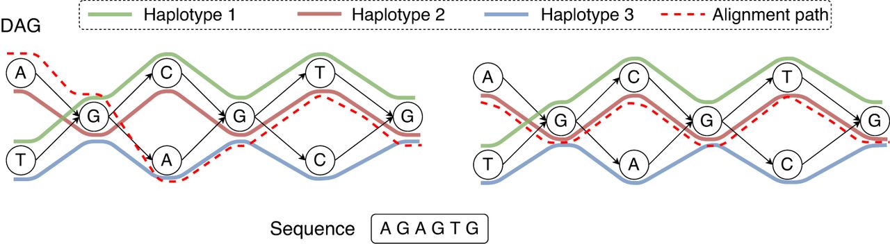
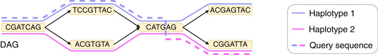
In this paper, we address the above limitations by introducing “haplotype-aware” formulations for (1) sequence-to-DAG alignment and (2) sequence-to-DAG chaining problems. Our formulations use the haplotype path information available in modern pangenome graphs. The formulations are inspired from the classic Li–Stephens haplotype copying model (Li and Stephens 2003). The Li–Stephens model is a probabilistic generative model that assumes that a sampled haplotype is an imperfect mosaic of known haplotypes. Similarly, our formulation for haplotype-aware sequence-to-DAG alignment problem optimizes the number of edits and haplotype switches simultaneously (Fig. 1). We give the $O (| Q | | E | | H |)$ time algorithm for solving the problem, where H denotes the set of haplotypes represented in the pangenome DAG. We further prove that the existence of a significantly faster algorithm than $O (| Q | | E | | H |)$ is not possible under the strong exponential time hypothesis (SETH) (Vassilevska Williams 2015). We also formulate the haplotype-aware colinear chaining problem. We solve it in $O (| H | N \log | H | N)$ time, assuming that a one-time preprocessing of the DAG is done in $O (| E | | H |)$ time. To provide evidence of the near optimality of this algorithm, we show that it is impossible to solve this problem significantly faster than $O (| H | N)$ under SETH.

Figure 1.

An example of an acyclic pangenome graph built using three haplotypes. The left figure shows the optimal alignment of the query sequence to the DAG with minimum edit distance. Accordingly, the edit distance is zero, and the count of recombinations is two. Next, suppose that we use recombination penalty −5 (formally defined in Methods). The right figure shows the new optimal alignment, where there is no recombination because the alignment path is consistent with haplotype 2.

Open in new tab Download PowerPointLink to figure

We implemented the proposed chaining algorithm in Minichain and evaluated it using simulated and real sequences. We built a pangenome DAG using 60 publicly available complete major histocompatibility complex (MHC) sequences (https://zenodo.org/records/6617246). We simulated query MHC haplotypes as mosaics of the 60 haplotypes. We demonstrate that introducing recombination penalty in the formulation leads to a much better consistency between the observed recombination events and the ground truth. We achieved Pearson's correlation up to 0.94 between the observed recombination count and the ground-truth recombination count, whereas the correlation remained below 0.23 if recombinations are not penalized.

We also tested Minichain using publicly available Pacific Biosciences (PacBio) and Oxford Nanopore Technologies (ONT) long reads from the CHM13 human genome (Vollger et al. 2020; Nurk et al. 2022). We demonstrate a better consistency between the ground-truth haplotype (CHM13) and the selected haplotype in the output. Our experiments suggest that haplotype-aware pattern-matching to pangenome graphs can be useful to improve read mapping and variant calling accuracy.

Methods

Haplotype-aware pangenome graphs and sequence alignments

First, we present the background concepts and notations before introducing our problem formulations and algorithms.

Haplotype-aware pangenome graph

Let $G (V, E, σ, H)$ be a DAG representing a pangenome reference. We assume that the DAG is weakly connected and |E| ≥ |V| − 1. Let Σ denote an alphabet. Function $σ : V \mapsto Σ$ assigns a character label to each vertex. $H = {H_{1}, H_{2}, \dots, H_{| H |}}$ denotes the set of haplotype sequences represented in the DAG. Each haplotype sequence can be identified using a path in the DAG. We define haps(v) as {i|H_i includes vertex v}. We assume that haps(v) ≠ ϕ for all v ∈ V and $h a p s (u) \cap h a p s (v) \neq ϕ$ for all edges (u, v) ∈ E. In other words, each vertex and edge must be supported by at least one haplotype. Given a query sequence Q ∈ Σ⁺, we will find its exact and approximate matches in the DAG. For brevity, we use [m] to denote the set {1, 2, …, m}, m ∈ ℕ. Let an alignment path of length l in the DAG be denoted as an ordered sequence (w₁, w₂, …, w_l), where each w_i is a pair of the form (v, h) such that v ∈ V, h ∈ haps(v), and (w_i.v, w_i+1.v) ∈ E for all i ∈ [l − 1]. Thus, in our haplotype-aware setting, an alignment path specifies a path in the DAG and the indices of the selected haplotypes along the path. We say that a recombination has occurred in between w_i and w_i+1 if w_i.h ≠ w_i+1.h. Given an alignment path P in the DAG, we use functions $s (P)$ and $r (P)$ to denote the sequence spelled by the path and the count of recombinations in the path, respectively.

Hardness result for the edit distance problem

Our hardness result (Lemma 3) will build on top of the seminal work of Backurs and Indyk (2015) . The orthogonal vector (OV) problem asks the following: given two sets of d-dimensional binary vectors A and B, |A| = |B| =: n, decide if there is a pair a ∈ A, b ∈ B such that a · b = 0. If the SETH (Vassilevska Williams 2015) holds and $d = ω (\log n)$ , there is no $ϵ > 0$ for which an $O (n^{2 - ϵ} poly (d))$ algorithm can solve the OV problem (Williams 2005). This result is frequently used to study the hardness of other problems (Backurs and Indyk 2015; Hoppenworth et al. 2020; Gibney et al. 2022; Equi et al. 2023a,b). For any two sequences P₁ and P₂, let EDIT(P₁, P₂) be the edit distance between them. Let us define another distance measure between two sequences as following:

PATTERN (P_{1}, P_{2}) = min_{x is a substring of P_{2}} EDIT (P_{1}, x) .

Backurs and Indyk (2015) proved the hardness of computing edit distance by designing two reductions: (1) OV to PATTERN and (2) PATTERN to EDIT. We recall the properties of their first reduction gadget.

Lemma 1

(Backurs and Indyk 2015): Given an OV problem instance with sets A = {a₁, …, a_n} and B = {b₁, …, b_n} comprising d-dimensional binary vectors, there exist transformations of sets A and B into two sequences S₁ and S₂, respectively, over the alphabet {0, 1, 2} such that the following properties hold:

– Computing PATTERN(S₁, S₂) determines the existence of orthogonal vectors. There exist constants β₁, β₂ ∈ ℕ such that if there is a pair of orthogonal vectors a ∈ A, b ∈ B, then PATTERN(S₁, S₂) ≤ β₁n − β₂; otherwise, PATTERN(S₁, S₂) = β₁n.
– |S₁| is a function of n and d. Similarly, |S₂| is a function of n and d. Both |S₁| and |S₂| are in O(n · poly(d)).
– Time to compute sequences S₁ and S₂ from sets A and B is in O(n · poly(d)).

We denote the injective function that generates the gadget sequence S₁ from set A as f₁. Similarly, injective function f₂ generates sequence S₂ from set B. The exact definitions of f₁ and f₂ are available elsewhere (Backurs and Indyk 2015).

Problem formulations for haplotype-aware sequence alignment

The input to each of the following problem is a DAG $G (V, E, σ, H)$ , a query Q ∈ Σ⁺, and a user-specified threshold k ∈ ℕ. In each problem, we seek a match of the query in the DAG while controlling the number of recombinations.

– Problem 1 (exact matching, limited recombinations): Determine if there is an alignment path P in DAG G such that $E D I T (s (P), Q) = 0$ and $r (P) < k$ .
– Problem 2 (approximate matching, no recombination): Determine if there is an alignment path P in DAG G such that $E D I T (s (P), Q) < k$ and $r (P) = 0$ .
– Problem 3 (approximate matching, limited recombinations): Let k, c₁, c₂ be user-specified thresholds, where k ∈ ℕ and c₁, c₂ ∈ ℝ ≥ 0. Here c₁ indicates cost per edit, and c₂ indicates cost per recombination. Determine if there is an alignment path P in DAG G such that $c_{1} \cdot E D I T (s (P), Q) + c_{2} \cdot r (P) < k$ .

In Problem 3, we assume a constant cost per recombination but one can also consider using different cost per locus based on known rates of recombination (Petes 2001). In the above set of problems, we have omitted the case with exact matching and no recombination. One way to solve this case is by doing exact sequence matching against each haplotype independently.

Proposed algorithms and theoretical analysis

Lemma 2:

Problems 1–3 can be solved in $O (| Q | | E | | H |)$ time.

Proof.

We show how to solve Problem 3 using dynamic programming. The same can be extended to Problems 1 and 2 as well. Our approach is similar to the standard sequence-to-DAG alignment algorithm (Lee et al. 2002) except that we also track recombinations. We add a dummy source vertex, $v_{ϵ}$ , with an empty label. It has zero incoming edges and |V| outgoing edges to all v ∈ V . Assume $h a p s (v_{ϵ}) = [| H |]$ . Let D(i, v, h) denote the minimum cost for aligning the (possibly empty) prefix of sequence Q ending at index i against an alignment path that ends at pair (v, h), $v \in V \cup {v_{ϵ}}, h \in h a p s (v)$ . We also maintain a second table, $D^{′′}$ , such that $D^{′′} (i, v)$ will store $min_{h \in h a p s (v)} D (i, v, h)$ . Initialize $D (0, v, h) = D^{′′} (0, v) = 0$ for all $v \in V \cup {v_{ϵ}}, h \in h a p s (v)$ . Initialize the remaining cells in table $D^{′′}$ to ∞. For $i \geq 1, v \in V \cup {v_{ϵ}}, h \in h a p s (v)$ , update D(i, v, h) and $D^{′′} (i, v)$ using the following recursion:

\begin{aligned} D (i, v, h) = min (D (i - 1, v, h) + c_{1}, \\ min_{\begin{matrix} (u, v) \in E, h^{'} \in h a p s (u), h^{'} = h \end{matrix}} {\begin{matrix} D (i, u, h^{'}) + c_{1} \\ D (i - 1, u, h^{'}) + c_{1} \cdot E D I T (σ (v), Q [i]) \end{matrix}, \\ min_{(u, v) \in E} {\begin{matrix} D^{′′} (i, u) + c_{1} + c_{2} \\ D^{′′} (i - 1, u) + c_{1} \cdot E D I T (σ (v), Q [i]) + c_{2} \end{matrix}), \\ D^{′′} (i, v) = min_{h^{'} \in h a p s (v)} D (i, v, h^{'}) . \end{aligned}

The recursion computes the optimal value of D(i, v, h) by considering the possibility of character deletion, insertion, match, and mismatch. The product c₁ · EDIT(σ(v), Q[i]) equals zero if there is a match between characters σ(v) and Q[i]. It equals c₁ in case of a mismatch. The other expressions involve addition of c₁ to consider the possibility of an insertion or a deletion. The expressions involving the addition of c₂ evaluate the possibility of a recombination. After updating D(i, v, h) for all h ∈ haps(v), we update

D^{′′} (i, v)

using the above equation. We compute values in table D in the increasing order of i and then the increasing topological order of

v \in V \cup {v_{ϵ}}

for a fixed i. The output, namely, the minimum alignment cost, is

min_{v \in V \cup {v_{ϵ}}} D^{′′} (| Q |, v)

. The runtime of the algorithm is dominated by the recursion. Solving the recursion takes

O (| Q | Σ_{v \in V \cup {v_{ϵ}}} (| h a p s (v) | \cdot (δ_{i n} (v) + 1)))

time, where δ_in(v) denotes the in-degree of vertex v. As a result, the time complexity of the algorithm is

O (| Q | | E | | H |)

Next, we prove that a significantly faster algorithm than $O (| Q | | E | | H |)$ for solving Problem 2 or 3 is unlikely. The existence of a faster algorithm for Problem 1 remains open.

Lemma 3:

For any constant $ϵ > 0$ , there is no algorithm that solves Problem 2 or Problem 3 in $O (| Q |^{1 - ϵ} | E | | H | + | Q | | E |^{1 - ϵ} | H | + | Q | | E |$ $| H |^{1 - ϵ})$ time, unless SETH is false.

Proof.

Problem 3 is a generalized version of Problem 2. Therefore, it suffices to prove the hardness of Problem 2. We derive the reduction from an OV problem. Suppose we have an OV instance with equal-sized sets A and B comprising d-dimensional binary vectors. Define n = |A| = |B|. We assume w.l.o.g. that n is a perfect square. We partition set A into $\sqrt{n}$ subsets $A_{1}, A_{2}, \dots, A_{\sqrt{n}}$ , each containing $\sqrt{n}$ vectors. Similarly, we partition set B into $\sqrt{n}$ subsets $B_{1}, B_{2}, \dots, B_{\sqrt{n}}$ , each containing $\sqrt{n}$ vectors. Observe that solving the OV problem for all (A_i, B_j) instances, $i, j \in [\sqrt{n}]$ , solves the OV problem for instance (A, B).

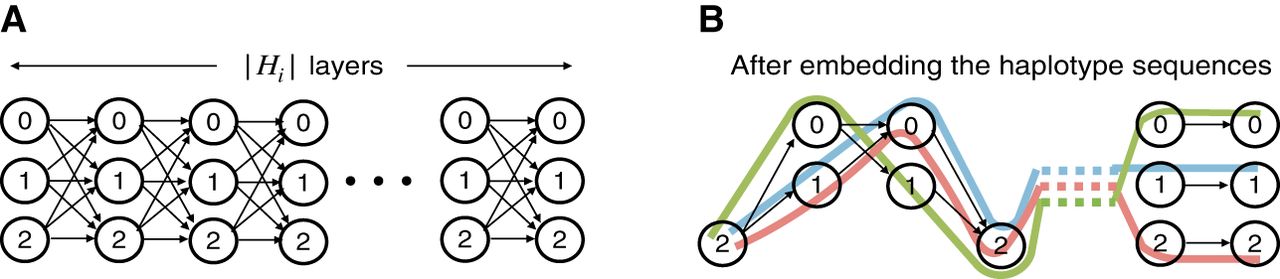
Next, we describe the construction of our gadget comprising query sequences $Q_{1}, \dots, Q_{\sqrt{n}}$ and haplotype-aware pangenome DAG $G (V, E, σ, H)$ . Assume the alphabet {0, 1, 2} for defining the query sequences and the vertex labels in the DAG. Define Q_i = f₁(A_i) for all $i \in [\sqrt{n}]$ (ref. Lemma 1). Next, we will construct $\sqrt{n}$ haplotype sequences. Define H_i = f₂(B_i) for all $i \in [\sqrt{n}]$ . Using Lemma 1, we know that all our haplotype sequences have uniform length; that is, $| H_{1} | = | H_{2} | = \dots = | H_{\sqrt{n}} |$ . Next, we construct a DAG where these haplotype sequences can be represented. We build a DAG with |H_i| “layers.” Each layer comprises three vertices labeled with characters “0,” “1,” and “2,” respectively (see Fig. 2A). Each layer (except the last) is fully connected to its next adjacent layer using 3² = 9 directed edges. Subsequently, we identify the unique path that spells each of the $\sqrt{n}$ haplotype sequences in this DAG. Finally, we discard the vertices and edges that are not used by any haplotype sequence (Fig. 2B).

Next, the above gadget will allow us to solve the OV problem by invoking the haplotype-aware sequence to graph alignment algorithm $\sqrt{n}$ times, once for each of the $\sqrt{n}$ query sequences. An alignment path with no recombination in the DAG spells a substring of a haplotype. Using Lemma 1, we make the following claim. There exist the two orthogonal vectors a ∈ A and b ∈ B if and only if we have at least one query sequence $q \in {Q_{1}, \dots, Q_{\sqrt{n}}}$ for which an alignment path P exists such that $r (P) = 0$ and $E D I T (s (P), q) < β_{1} \sqrt{n}$ . It is only remaining to show that a faster algorithm for Problem 2 will contradict SETH by enabling a faster algorithm for the OV problem. Observe that (1) each |Q_i| and |H_i| is in $O (\sqrt{n} \cdot poly (d))$ ; (2) |V| and |E| are asymptotically equal to |H_i|; (3) number of haplotypes is $| H | = \sqrt{n}$ ; and (4) we invoke the alignment algorithm $\sqrt{n}$ times. Construction of the gadget requires O(n · poly(d)) time. Therefore, if Problem 2 can be solved in $O (| Q |^{1 - ϵ} | E | | H | + | Q | | E |^{1 - ϵ} | H | + | Q | | E | | H |^{1 - ϵ})$ time for some $ϵ > 0$ , then the OV problem can be solved in $O (n^{2 - ϵ / 2} \cdot poly (d))$ time.

Figure 2.

An illustration of the pangenome DAG used in the reduction proof of Lemma 3. An initial version of the DAG (A) and the changes made after addition of all the haplotype paths (B).

Open in new tab Download PowerPointLink to figure

Methods for haplotype-aware chaining on graphs

Most alignment tools use a seed-chain-extend heuristic to compute the alignments quickly (Sahlin et al. 2023; Shaw and Yu 2023). Given a set of seed matches (anchors) as input, colinear chaining is a rigorous optimization technique to identify promising alignment regions in a reference. It identifies a coherent subset of anchors such that their coordinates are ordered on the query and the reference. The selected anchors are subsequently combined together to form an alignment. Several versions of colinear chaining problems have been studied for aligning two sequences (Eppstein et al. 1992a,b; Myers and Miller 1995; Abouelhoda and Ohlebusch 2005; Otto et al. 2011; Mäkinen and Sahlin 2020; Jain et al. 2022). Recent works have further studied the extension of chaining on acyclic (Mäkinen et al. 2019; Chandra and Jain 2023; Ma et al. 2023; Rizzo et al. 2023a) and cyclic pangenome graphs (Antipov et al. 2016; Rajput et al. 2024), but these formulations do not consider the haplotype paths.

Concepts and notations for haplotype-aware colinear chaining

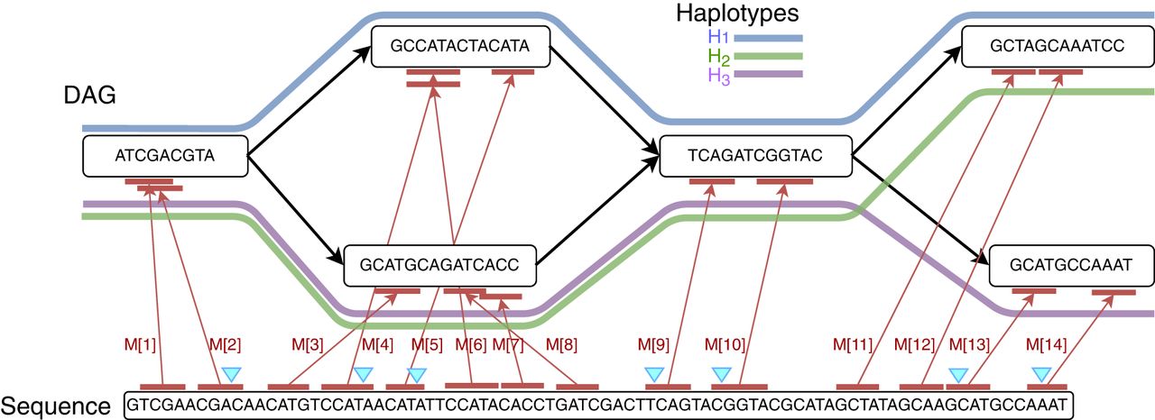
From here on, we assume that vertices of a haplotype-aware pangenome DAG are labeled with sequences. Sequence-labeled vertices permit a more compact graph representation, which will be useful in the context of chaining. It is trivial to transform a graph from sequence-labeled form to character-labeled form and vice versa. Let function σ:V → Σ⁺ label each vertex v ∈ V with sequence σ(v) in DAG $G (V, E, σ, H)$ . The input to the chaining problem is a set of anchors, {M[1], M[2], …, M[N]}. An anchor is represented by a three-tuple (v, [x..y], [c..d]), which signifies a match between query substring Q[c..d] and substring σ(v)[x..y] in the DAG (Fig. 3). The weight function assigns a user-specified weight to each anchor. Anchor weights are typically set proportional to the length of the matching substrings in practice. We use R⁻(v)⊆ V to denote the subset of vertices that can reach v using a path in the DAG. Vertex v is also included in R⁻(v). Next, we define the precedence relationship between a pair of anchors.

Figure 3.

An example that shows anchors (in red) between a query sequence and a pangenome DAG. The DAG comprises three haplotype sequences, H₁, H₂, H₃. In this example, the ordered sequence of pairs [(2, 1), (4, 1), (5, 1), (9, 1), (10, 1), (13, 3), (14, 3)] forms a chain, and the corresponding anchors are highlighted using blue markers. This chain includes a single recombination.

Open in new tab Download PowerPointLink to figure

Definition 1 (precedence).

Given two anchors M[i] and M[j], M[i] precedes (≺) M[j] if (1) M[i].d < M[j].c, (2) M[i].v ∈ R⁻(M[j].v), and (3) M[i].y < M[j].x if M[i].v = M[j].v.

Definition 2 (chain).

A chain is an ordered sequence (s₁, s₂, …, s_p), where each s_j is a pair of the form (i, h) such that i ∈ [N], h ∈ haps(M[i].v), and $M [s_{j} . i] ≺ M [s_{j + 1} . i]$ for all j ∈ [p − 1].

In our definition, a chain specifies the indices of the selected haplotypes alongside the anchors (Fig. 3). For the sake of efficiency, our precedence condition does not permit overlap between adjacent anchors in a chain. We say that a recombination has occurred in between s_j and s_j+1 if s_j.h ≠ s_j+1.h. Given a chain S, we use the function r(S) to denote the count of recombinations in S. Let γ ∈ ℝ_≥0 be a user-specified parameter that specifies cost per recombination.

Similar to work by Mäkinen et al. (2019), we will use a path cover to facilitate efficient sparse dynamic programming on the DAG. A path cover is a set of paths in the DAG such that every vertex in V is included in at least one path. Previous chaining algorithms (see, e.g., Mäkinen et al. 2019; Chandra and Jain 2023; Ma et al. 2023) identify a path cover with the minimum number of paths because the runtime of sparse dynamic programming increases with the size of the path cover (Mäkinen et al. 2019). In the haplotype-aware setting, we will directly use the paths corresponding to the haplotype sequences as path cover. Let $P_{1}, P_{2}, \dots, P_{| H |}$ be the paths corresponding to the haplotype sequences $H_{1}, H_{2}, \dots, H_{| H |}$ , respectively. ${P_{1}, P_{2}, \dots, P_{| H |}}$ is a path cover of the DAG because each vertex in the DAG is included in at least one haplotype (Methods subsection “Haplotype-aware pangenome graph”). Suppose $l a s t 2 r e a c h (v, h), v \in V, h \in [| H |]$ denotes the last vertex in path P_h that belongs to R⁻(v). last2reach(v, h) does not exist if no vertex in path P_h can reach vertex v. We precompute last2reach(v, h) for all v ∈ V and $h \in [| H |]$ in $O (| E | | H |)$ time by using the algorithm from Mäkinen et al. (2019). This is a one-time preprocessing step that will be useful to solve the chaining problems efficiently. Next, we also use the following standard data structure in our chaining algorithm.

Lemma 4

(Mäkinen et al. 2015): Let n be the number of leaves in a tree, each storing a (key, value) pair. The data structure uses a balanced binary search tree. It supports update and range maximum query (RMQ) operations, defined below, in $O (\log n)$ time:

– update(k, val): For the leaf w with key = k, $v a l u e (w) \leftarrow max (v a l u e (w), v a l)$ .
– RMQ(l, r): Return $max {v a l u e (w) | l < k e y (w) < r}$ .

Given n (key, value) pairs, the tree can be constructed in $O (n \log n)$ time and O(n) space.

Problem formulations for haplotype-aware colinear chaining

– Problem 4 (limited recombinations): Determine an optimal chain S = s₁, s₂, …, s_p that maximizes the chaining score, defined as $\sum_{j = 1}^{p} w e i g h t (M [s_{j} . i]) - γ \cdot r (S)$ .

The second term γ · r(S) in the above scoring function corresponds to the penalty for haplotype switches in a chain. While scoring a chain, it is also essential to penalize the gap corresponding to the distance (in base pairs) between adjacent pair of anchors. Accordingly, we formulate a gap-sensitive version of the above problem. We assume the same definition of function gap(M[i], M[j]), i, j ∈ [N] as used by Chandra and Jain (2023); see Problem 2a in their paper.

– Problem 5 (limited recombinations, gap-sensitive): Determine an optimal chain S = s₁, s₂, …, s_p that maximizes the chaining score, defined as $\sum_{j = 1}^{p} w e i g h t (M [s_{j} . i]) - \sum_{j = 2}^{p} g a p (M [s_{j - 1} . i], M [s_{j} . i]) -$ $γ \cdot r (S)$ .

Proposed chaining algorithms and theoretical analysis

First, it is useful to discuss a simple dynamic programming solution for Problem 4. Let C(i, h) denote the optimal score of a chain ending at pair (i, h), where i ∈ [N], h ∈ haps(M[i].v). We use $C^{′′} (i)$ to store max_{h∈haps(M[i].v)}C(i, h). A single anchor is a valid chain of size one; therefore, we initialize C(i, h) to weight(M[i]) for all i ∈ [N], h ∈ haps(M[i].v). Also, initialize $C^{′′} (i)$ to weight(M[i]) for all i ∈ [N]. We update C(i, h) to its optimal value using the following recursion:

\begin{aligned} C (i, h) = max (w e i g h t (M [i]), \\ max_{\begin{matrix} M [k] ≺ M [i], h^{'} \in h a p s (M [k] . v), \\ h^{'} = h, k \in [N] \end{matrix}} C (k, h^{'}) + w e i g h t (M [i]), \\ max_{M [k] ≺ M [i], k \in [N]} C^{′′} (k) + w e i g h t (M [i]) - γ), \\ C^{′′} (i) = max_{h^{'} \in h a p s (M [i] . v)} C (i, h^{'}) . \end{aligned}

M [k] ≺ M [i]

and path P_h covers both the vertices M[k].v and M[i].v, then the chaining score obtained using C(k, h) is considered without recombination penalty. The third term in the expression considers the score with recombination penalty γ. This is needed when

(k, h^{'})

h^{'} \neq h

precedes (i, h). After updating C(i, h) for all h ∈ haps(M[i].v), we also update

C^{′′} (i)

using the above equation. Let function rank(v) specify the topological ordering of vertex v in the DAG. The C(i, h) values should be computed in lexicographically ascending order based on the key (rank(M[i].v), M[i].x). For a fixed i, C(i, h) values may be computed in any order. The above algorithm fills up to

| H | N

values in table C. Computing each value using a linear scan would require considering all N number of anchors and filtering those that satisfy the precedence criteria. Even if we ignore the time for filtering and checking precedence, the worst-case asymptotic runtime of this algorithm grows at least as fast as

| H | N^{2}

. This makes it too slow when N is in millions, which typically happens when aligning megabase-long de novo assembled sequences to human pangenome DAGs. To address this, we propose a faster

O (| H | N \log | H | N)

time algorithm for solving Problem 4. First, we note the following inequality.

Lemma 5:

$C (i, h) \geq C^{′′} (i) - γ$ for all i ∈ [N], h ∈ haps(M[i].v).

Proof.

Consider any value of i ∈ [N] and h ∈ haps(M[i].v). Let $h^{'} = argma x_{k \in h a p s (M [i] . v)} C (i, k)$ , breaking ties arbitrarily if necessary. Then, $C^{′′} (i)$ equals $C (i, h^{'})$ . If $h^{'} = h$ , then $C (i, h) = C^{′′} (i)$ ; thus, the inequality holds. Next, consider the case when $h^{'} \neq h$ . Let S₁ = s₁, s₂, …, s_p−1, s_p be an optimal chain that ends at pair $(i, h^{'})$ . We consider another chain, $S_{2} = s_{1}, s_{2}, \dots, s_{p - 1}, {s_{p}}^{'}$ , such that ${s_{p}}^{'} = (i, h)$ . Suppose the score of chain S₂ is x. Both chains S₁ and S₂ differ only by the haplotype used in their last pairs. Therefore, the difference in the chaining scores of S₁ and S₂ is at most γ (one recombination). Thus, $x \geq C^{′′} (i) - γ$ . Also, C(i, h) must be ≥x.

Lemma 6:

Assuming DAG $G (V, E, σ, H)$ is preprocessed, Problem 4 can be solved in $O (| H | N \log | H | N)$ time.

Proof.

See Algorithm 1 for an outline of our approach. We extend the sparse dynamic programming framework of Mäkinen et al. (2019) to our haplotype-aware setting. Our path cover ${P_{1}, P_{2}, \dots, P_{| H |}}$ contains $| H |$ paths corresponding to the $| H |$ haplotype sequences. We use $| H |$ search trees $T_{1}, T_{2}, \dots, T_{| H |}$ , one per path. Each search tree $T_{h}$ will record C(i, h) scores specific to that haplotype.

Algorithm 1

O (| H | N \log | H | N)

time chaining algorithm for Problem 4

Input: Weighted anchors M[1..N], haplotype paths $P_{1}, P_{2}, \dots, P_{| H |}$ , last2reach values, parameter γ

Output: Table C such that C(i, h)= optimal score of a chain that ends at (i, h), for all $i \in [N], h \in [| H |]$

1 Initialize search trees $T_{h}$ , for all $h \in [| H |]$ , using keys {M[i].d|1 ≤ i ≤ N} and values −∞

2 Initialize $C (i, h), C^{′′} (i)$ and C_l2r(i) as weight(M[i]), for all $i \in [N], h \in [| H |]$

3 /* Create array Z that stores tuples of the form (v, pos, task, anchor, haplotype), where v ∈ V, pos ∈ ℕ, task ∈ {0, 1, 2}, anchor ∈ [N], and $h a p l o t y p e \in [| H |]$ .*/

4 for i ← 1 to N do

5 for $h \leftarrow 1 t o | H |$ do

6 if h ∈ haps(M[i].v) then

7 Z.push(M[i].v, M[i].x, 0, i, h)

8 Z.push(M[i].v, M[i].x, 1, i, h)

9 Z.push(M[i].v, M[i].y, 2, i, h)

10 else if last2reach(M[i].v, h) exists then

11 $v_{l 2 r} \leftarrow l a s t 2 r e a c h (M [i] . v, h)$

12 $Z . p u s h (v_{l 2 r}, | σ (v_{l 2 r}) | + 1, 0, i, h)$

13 end

14 end

15 for z ∈ Z in lexicographically ascending order based on the key (rank(v), pos, task) do

16 i ← z.anchor, h ← z.haplotype, v ← z.v, wt ← weight(M[i])

17 if z.task = 0 then

18 if h ∈ haps(M[i].v) then

19 $C (i, h) \leftarrow max (C_{l 2 r} (i), C (i, h), w t + T_{h} . RMQ (0, M [i] . c))$

20 $C^{′′} (i) \leftarrow max (C^{′′} (i), C (i, h))$

21 else

22 $C_{l 2 r} (i) \leftarrow max (C_{l 2 r} (i), w t + T_{h} . RMQ (0, M [i] . c) - γ)$

23 else if z.task = 1 then

24 $C (i, h) \leftarrow max (C^{′′} (i) - γ, C (i, h))$

25 else if z.task = 2 then

26 $T_{h} . update (M [i] . d, C (i, h))$

27 end

We initialize each search tree with keys {M[i].d |1 ≤ i ≤ N} and values −∞ (Line 1). In Lines 4–13, we create an array Z with $O (| H | N)$ tuples. After sorting of Z (Line 15), these tuples ensure that the search trees are updated and queried in a proper order. At the time of processing C(i, h), i ∈ [N], h ∈ haps(M[i].v), the algorithm would have already finished processing $C (k, h^{'})$ for all $k, h^{'}$ such that $M [k] ≺ M [i], h^{'} \in h a p s (M [k] . v)$ . The score $C (k, h^{'})$ would have already been recorded in search tree $T_{h^{'}}$ (Line 26).

All the anchors that lack a preceding anchor are optimally processed at the initialization stage (Line 2). Suppose an optimal chain ending at (i, h) is s₁, s₂, …, s_p−1, s_p such that $s_{p - 1} = (k, h^{'})$ and s_p = (i, h). Assume that $C (k, h^{'})$ is already computed optimally. While calculating C(i, h), the algorithm handles the following three cases:

– (Case 1) $h = h^{'}$ : In this case, we optimally compute C(i, h) by executing a range query in search tree T_h (Line 19). Because $M [k] ≺ M [i]$ and $h^{'} = h$ , search tree T_h returns the value $C (k, h^{'})$ stored in key M[k].d.
– (Case 2) $h \neq h^{'}$ , and path $P_{h^{'}}$ does not cover M[i].v: Observe that $l a s t 2 r e a c h (M [i] . v, h^{'})$ must exist in this case because M[k].v must reach M[i].v. In Lines 10–12, we add tuples in array Z to ensure that C_l2r(i) is updated by using a range query in search tree $T_{h^{'}}$ (Line 22). We also put a penalty γ owing to recombination in this case. This update to C_l2r(i) happens after all anchors in vertex $l a s t 2 r e a c h (M [i] . v, h^{'})$ have been processed and search tree $T_{h^{'}}$ has been updated because of our definition and ordering of the tuples in array Z (Lines 12, 15). Later when we update C(i, h) in Line 19, it gets its optimal value using C_l2r(i).
– (Case 3) $h \neq h^{'}$ , and path $P_{h^{'}}$ covers M[i].v: If $(s_{1}, s_{2}, \dots, (k, h^{'}), (i, h))$ is an optimal chain ending at (i, h), then $(s_{1}, s_{2}, \dots, (k, h^{'}), (i, h^{'}))$ must be an optimal chain that ends at $(i, h^{'})$ . Accordingly, $C (i, h^{'}) = C (i, h) + γ$ . It implies $C^{′′} (i) \geq C (i, h) + γ$ . Using the inequality in Lemma 5, we get $C (i, h) = C^{′′} (i) - γ$ . Accordingly, C(i, h) is updated to its optimal value in Line 24.

The total runtime of the algorithm is dominated by sorting of array Z. Sorting an array of size $O (| H | N)$ takes $O (| H | N \log | H | N)$ time. Initializing $| H |$ search trees takes $O (| H | N \log N)$ time. The algorithm uses $O (| H | N)$ number of $O (\log N)$ -time RMQ and update operations on the search trees (Lemma 4).

In the above algorithm, the optimal chain can be obtained easily by adding backtracking pointers. We next show that any algorithm to solve Problem 4 has a time complexity that is not polynomially faster than $O (| H | N)$ under SETH.

Lemma 7:

For any constant $ϵ > 0$ , there is no algorithm that solves Problem 4 in $O (| H |^{1 - ϵ} N + | H | N^{1 - ϵ})$ time unless SETH is false.

Proof.

The reduction from the OV problem is as follows. Suppose an OV instance is given as A = {a₁, …, a_n} and B = {b₁, …, b_n} and each set is comprised of d-dimensional binary vectors.

We perform this reduction by constructing a haplotype-aware graph based on A and a sequence based on B with anchors such that there is an anchor chain of some desired value if and only if there is an orthogonal pair of vectors. The main intuition is that an orthogonal pair of vectors should allow a high-value portion of the chain between the corresponding vector gadgets, whereas the remaining vector gadgets can be used in some portion of the chain and give a predictable value.

To this end, we first define component gadgets:

C G (0) = 000 C G (1) = 001.

We use

◯_{i = 1}^{d} s_{i}

to denote the concatenation of sequences s₁, …, s_d and

s_{1} \circ s_{2}

to denote the concatenation of two sequences, s₁ and s₂. For a symbol c and an integer i, we use cⁱ to denote symbol c repeated i times. Using the above component gadgets, we define our vector gadgets:

V G (a_{i}) = ◯_{x = 1}^{d} C G (a_{i} [x]) V G (b_{i}) = ◯_{x = 1}^{d} C G (b_{i} [x]) .

The query sequence is defined as

Q = ◯_{i = 1}^{n} V G (b_{i})

. For 1 ≤ i ≤ n, we construct haplotype sequence H_i from vector a_i:

H_{i} = 0^{n d} \circ V G (a_{i}) \circ 0^{n d} .

To create the vertices of graph G, we start with the following: a vertex denoted v_left with label 0^nd; 2d vertices denoted v_x,0, v_x,1 for 1 ≤ x ≤ d, where each v_x,0 has label CG(0) and each v_x,1 has label CG(1); and a vertex denoted v_right with label 0^nd. For edges, we add edges from v_left to v_1,0 and from v_left to v_1,1; for 1 ≤ x < d, we add edges from v_x,0 to v_x+1,0 and v_x+1,1 and from v_x,1 to v_x+1,0 and v_x+1,1; and we then add edges from v_d,0 to v_right and from v_d,1 to v_right. Next, we embed each haplotype in G by following its only possible path from v_left to v_right and deleting any vertices and edges not supported by some haplotype. See Figure 4. We call the subgraph of G excluding only v_left and v_right the center of G.

Figure 4.

Reduction from OV problem with sets A = {0110, 1100, 1101} and B = {1010, 1001, 1011}.

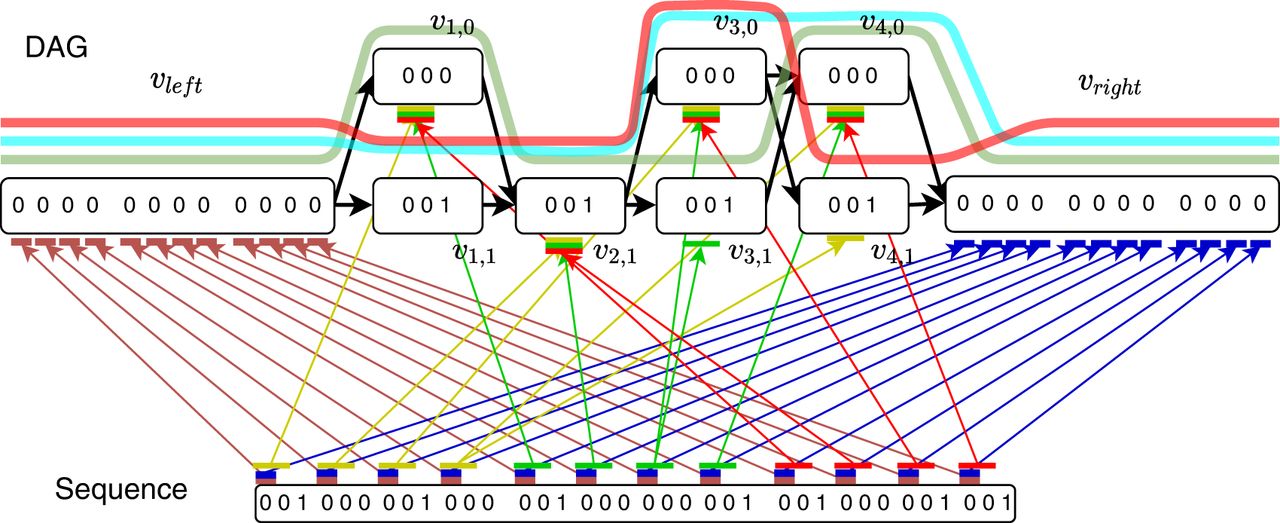
Open in new tab Download PowerPointLink to figure

The anchors are described next. For all i ∈ [n] and for all x ∈ [d], we define the following weight-1 anchors:

\begin{aligned} M_{i, x}^{l e f t} & = (v_{l e f t}, [(i - 1) d + x . . (i - 1) d + x], \\ [3 (i - 1) d + 3 (x - 1) + 1..3 (i - 1) d + 3 (x - 1) + 1]) \end{aligned}

We similarly define weight-1 anchors:

\begin{aligned} M_{i, x}^{r i g h t} & = (v_{r i g h t}, [(i - 1) d + x . . (i - 1) d + x], \\ [3 (i - 1) d + 3 (x - 1) + 1..3 (i - 1) d + 3 (x - 1) + 1]) . \end{aligned}

For all i ∈ [n] and for all x ∈ [d], if b_i[x] = 0 and if v_x,0 and v_x,1 exist, we define the following weight-2 anchors

M_{i, x, 0}^{c e n t e r} = (v_{x, 0}, [1..2], [3 (i - 1) d + 3 (x - 1) + 1..3 (i - 1) d + 3 (x - 1) + 2])

M_{i, x, 1}^{c e n t e r} = (v_{x, 1}, [1..2], [3 (i - 1) d + 3 (x - 1) + 1..3 (i - 1) d + 3 (x - 1) + 2]) .

If either v_x,0 or v_x,1 do not exist, we omit the corresponding anchor. If b_i[x] = 1 and v_x,0 exists, we define the following weight-2 anchor:

M_{i, x, 0}^{c e n t e r} = (v_{x, 0}, [1..2], [3 (i - 1) d + 3 (x - 1) + 1..3 (i - 1) d + 3 (x - 1) + 2]) .

We set the recombination penalty γ = 1. We show the correctness of the above reduction in Lemmas 8–11.

Lemma 8:

If there exists an orthogonal pair a_i ∈ A and b_j ∈ B, then there exists an anchor chain with cost 2d + (n − 1)d.

Proof.

First take anchors $M_{j^{'}, x}^{l e f t}$ for $1 \leq j^{'} < j$ , 1 ≤ x ≤ d. This part of the chain has a value of (j − 1)d. Next, for 1 ≤ x ≤ d, if a_i[x] = 0 and b_j[x] = 0 or a_i[x] = 0 and b_j[x] = 1, take $M_{j, x, 0}^{c e n t e r}$ ; if a_i[x] = 1 and b_j[x] = 0, take $M_{j, x, 1}^{c e n t e r}$ . This part of the chain has a value of 2d. Lastly, for $j^{'} > j$ , 1 ≤ x ≤ d, take anchors $M_{j^{'}, x}^{r i g h t}$ ; this part of the chain has value (n − j)d. This forms a valid chain and requires no recombinations. Thus, the total score is (j − 1)d + 2d + (n − j)d = 2d + (n − 1)d.

Lemma 9:

If a chain exists with score 2d + (n − 1)d, then in this chain, no recombinations are used, and anchors starting at all the anchor starting positions in Q are used.

Proof.

For a given x, only one anchor to either v_x,0 or v_x,1 can be used while maintaining the precedence condition. Because each anchor to the center of G has a weight of two, the total contribution of the center of G to the score is at most 2d. The remaining anchors in the chain have a weight of one, and there are at most (n − 1)d of them after d anchors are used in the center. Hence, the maximum possible score is 2d + (n − 1)d. Notice also that taking d anchors in the center is the only way to achieve such a score.

The claim that there are no recombinations follows, as the maximum possible score using recombination becomes 2d + (n − 1)d − 1. The second claim follows because any chain using fewer than dn anchors cannot achieve the maximum score of 2d + (n − 1)d.

Lemma 10:

If a chain exists with the score 2d + (n − 1)d, then in this chain, all anchors for some vector gadget in Q are to the center of G.

Proof.

If anchors from two different vector gadgets in Q are to the center of G, then because the center is contributing 2d to the score (the only way a score of 2d + (n − 1)d is achieved), there must be anchors M and $M^{'}$ from two different vector gadgets that occur in adjacent vertices in the center, say with $M ≺ M^{'}$ . However, this implies that there are at least d − 1 anchor positions in Q between M and $M^{'}$ are not used in the solution, contradicting Lemma 9.

Lemma 11:

If there exists a chain with score 2d + (n − 1)d, then there exists orthogonal vectors a_i and b_j.

Proof.

By Lemma 10, some vector gadget VG(b_j) has all of its anchors going to the center of G. By Lemma 9, no recombinations are used, and these must lie on some path for a haplotype constructed from a vector a_i. By design of the component gadgets, for 1 ≤ x ≤ d if a_i[x] = 1 we get an anchor between v_x,1 on the haplotype path for a_i and VG(b_j) if and only if b_j[x] = 0. We conclude that a_i and b_j are orthogonal.

Observe that the total number of M^left anchors is dn, the total number of M^right anchors is dn, and the total number of M^center anchors is at most 2dn; thus, N = O(dn). The number of haplotypes is $| H | = n$ . Furthermore, |Q| = O(dn) and the graph G has O(d) vertices and edges, and the sum of vertex label lengths is O(dn). Hence, the reduction takes O(dn) time. Combined with Lemmas 8 and 11, it follows that an algorithm for Problem 4 running in time $O (| H |^{1 - ϵ} N + | H | N^{1 - ϵ})$ solves the OV problem in time $O (n^{2 - ϵ} \cdot poly (d))$ . This completes the proof of Lemma 7.

Problem 5 can be solved by extending Algorithm 1 (Supplemental Note S1). The extension requires a few additional terms corresponding to gap cost between adjacent anchors. This algorithm also runs in $O (| H | N \log | H | N)$ time. The reduction presented in Lemma 7 can be easily extended for Problem 5 as well.

Implementation and benchmarking details

Software implementation

We implemented Algorithm 1 and the modifications to include gap penalty (for description, see Supplemental Note S1). We added our implementation in the Minichain code (Chandra and Jain 2023). Our new chaining implementation replaces the haplotype-agnostic chaining implementation proposed in our previous work. Minichain supports an end-to-end seed-chain-extend workflow to align long reads and contigs to acyclic pangenome graphs. Similar to the previous version of the software, we use the seeding and base-to-base alignment routines from Minigraph (Li 2018). We leave the implementation of our $O (| Q | | E | | H |)$ time base-to-base alignment algorithm (Methods) as future work because it requires further practical optimizations to reduce the runtime, for example, using banded alignment or wavefront heuristics (Rautiainen and Marschall 2020; Marco-Sola et al. 2021; Zhang et al. 2022).

In Minichain, we parse the set of vertices, edges, and haplotype paths from a graphical fragment assembly (GFA) file (https://github.com/GFA-spec/GFA-spec). A read may be sampled from the same or the opposite orientation with respect to the graph. Accordingly, for each connected component in the input graph, we create another component of the same size with reverse-complemented vertex labels and reversed edges. We use the same path cover for the second component as the original component, but the direction of each path is reversed. We compute anchors by using Minigraph's seeding method, which finds (w, k)-minimizer matches (Roberts et al. 2004) between the query sequence Q and the vertex string labels σ(v) for all v ∈ V. The default values of w and k are 11 and 17, respectively. We set the weight of each anchor as 200 · k by default based on our experimental observations. Thus for k = 17, each anchor in a chain contributes 3400 to the total chain score. The multiplicative factor of 200 prevents gap penalties to dominate the overall chain score. Minichain can report multiple best-scoring chains and assign a mapping quality (Li et al. 2008) to each chain; the criteria for this remains same as before (Chandra and Jain 2023). We evaluate the chains produced by our algorithm without subjecting it to further Minigraph's heuristics.

Pangenome graph construction

We used 60 publicly available complete MHC haplotype sequences (https://zenodo.org/records/6617246). This set of 60 MHC haplotype sequences is composed of the CHM13 MHC haplotype (Nurk et al. 2022) and 59 other haplotypes from the Human Pangenome Reference Consortium (Liao et al. 2023). The length of these sequences varies from 4.8 Mbp to 5.1 Mbp. The MHC region is known to have significant polymorphism, inter-gene sequence similarity, and long-range haplotype structures (Dilthey 2021). We used Minigraph (v0.20-r559) (Li et al. 2020) to build an acyclic pangenome graph using the 60 MHC haplotypes. The graph construction algorithm in Minigraph augments structural variants (SVs) of size ≥50 bp in the graph. Our MHC pangenome graph contains 984 vertices, 1387 edges, and 210 SVs. Because Minigraph does not output haplotype paths in the graph, we realigned each haplotype to the graph to obtain the corresponding paths.

Simulation of query sequences

We simulated 135 MHC haplotype sequences. Each sequence was simulated as an imperfect mosaic of the 60 reference haplotypes (Fig. 5). We used the following procedure for simulation: (1) select a random haplotype path in the graph; (2) read the first l bases from the chosen haplotype path in the graph; (3) if the (l + 1)^th base is in vertex v and |haps(v)| ≥ 2, then switch to another randomly chosen haplotype path at vertex v; and (4) read the next l bases, and repeat the procedure until we hit the last base of a haplotype path. After generating a sequence, we added substitutions at randomly chosen loci in the sequence. These substitutions approximately mimic true mutations and sequencing errors in real data. For each substitution rate of 0.1%, 1%, and 5%, we simulated 45 sequences. In each case, three sets of 15 sequences were simulated using l = 1 Mbp, l = 2 Mbp, and l = 3 Mbp, respectively. Using this procedure, the number of recombination events in all the simulated sequences ranged from one to four. Our pangenome graph and the set of query sequences are available on Zenodo (https://doi.org/10.5281/zenodo.10665350).

Figure 5.

An example to illustrate simulation of a query sequence as a mosaic of reference haplotypes. In this example, l = 19.

Open in new tab Download PowerPointLink to figure

Results

Comparison with haplotype-agnostic chaining using simulated data

We demonstrate that integrating recombination penalty in the sequence-to-graph chaining problem formulation leads to an improved concordance of the haplotypes used in our chains and the ground truth. A positive finite recombination penalty in our problem formulation allows the user to limit the recombinations in an optimal chain. If we set recombination penalty γ = 0, then our algorithm is equivalent to the haplotype-agnostic chaining algorithm of Chandra and Jain (2023). Recombination penalty γ = ∞ corresponds to haplotype-restricted chaining, where a chain can use only one of the reference haplotypes. We evaluated Minichain by using simulated MHC haplotype sequences and different values of recombination penalty γ = 0, 10³, 10⁴, 10⁵, 10⁶, ∞. Minichain computes an optimal chain as a sequence of pairs of the selected anchors and the haplotype indices. Thus, we know the sequence of haplotype indices and the number of recombinations in each chain.

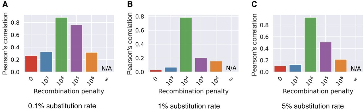
We show the Pearson correlation coefficients between the observed number of recombinations and the true number of recombinations using different values of substitution rates and recombination penalties (Fig. 6A–C). The results suggest that γ = 10⁴ gives the best correlation across different substitution rates. The correlation is weak when γ = 0 or γ = 10⁶. The correlation is not defined when γ = ∞ because the observed number of recombinations remained zero; thus, the standard deviation of the observed values remained zero. In the haplotype-agnostic setting (γ = 0), a highest-scoring chain of minimizers can contain incorrect haplotype switches (for an example, see Supplemental Fig. S1). γ = 10³ is also too low for setting recombination penalty because a single anchor in a chain contributes 3400 to the chaining score (Methods), and the algorithm may still favor an additional anchor even if it involves an incorrect haplotype switch. Using γ ≥ 10⁴, the recombination penalty equals the score contributed by three or more anchors.

Figure 6.

Pearson's correlation between the number of recombinations in Minichain's output chain and the true count. We evaluated the performance with substitution rates 0.1% (A), 1% (B), and 5% (C) and different recombination penalties.

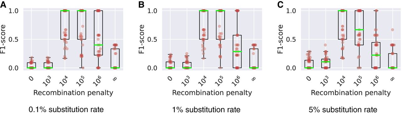
Open in new tab Download PowerPointLink to figure

Next, we compared the list of query sequences’ source haplotypes to the selected haplotypes in the output chains. Suppose a query sequence was simulated using haplotypes in the order $H_{i_{1}}, H_{i_{2}}, \dots, H_{i_{n}}$ ; then, we recorded the “true haplotype recombination pairs” as a set of pairs ${(s t a r t, H_{i_{1}}), (H_{i_{1}}, H_{i_{2}}), \dots, (H_{i_{n - 1}}, H_{i_{n}}), (H_{i_{n}}, e n d)}$ . Similarly, we recorded the sets corresponding to the “observed haplotype recombination pairs” from Minichain's output chains. We compared these two sets for each query and calculated the F1-scores (Fig. 7A–C; Supplemental Fig. S4; Supplemental Table S1). In this experiment, precision was determined by the fraction of observed recombination pairs that were in the true set. Similarly, recall was determined by the fraction of true recombination pairs that was observed in the output. We achieved higher F1-scores with γ = 10⁴, 10⁵ compared with the haplotype-agnostic (γ = 0) and haplotype-restricted (γ = ∞) modes. These results suggest that haplotype-aware chaining and alignment algorithms can be useful to prevent spurious recombinations.

Figure 7.

Box plots show the levels of consistency between the haplotype recombination pairs in Minichain's output chain and the ground truth using three different sets of simulated MHC sequences with substitution rates 0.1% (A), 1% (B), and 5% (C). We tested using different recombination penalties. Each red dot in the plots corresponds to a query sequence. The median values are highlighted in green.

Open in new tab Download PowerPointLink to figure

We restricted the maximum count of recombinations in the simulated MHC haplotypes to four in the above experiments because MHC sequences are known to have long-range haplotype structures (Dilthey 2021). We performed additional experiments with higher number of recombination events (range: three to nine) and reached similar conclusions (Supplemental Figs. S2, S3).

Our MHC pangenome graph comprises SVs only. We expect further improvements in the accuracy of our algorithm if substitution and short indel variation are also augmented in a pangenome graph (Hickey et al. 2024). This is because more variants will help to distinguish between near-identical or closely related haplotypes. Doing this will also require improvements in Minichain's seeding and chaining implementation to allow the use of anchors that cover small bubbles in a graph. This is possible by considering a more flexible definition of anchors that can span multiple vertices (Rossi et al. 2022; Rizzo et al. 2023a,b). Our implementation uses minimizers, which also have a known weakness of being context dependent; that is, the decision to sample a k-mer is made based on its neighboring k-mers (Edgar 2021).

The runtime of Minichain ranged from 5 to 11 min for aligning a simulated MHC sequence to the pangenome graph. The worst-case time complexity of the proposed haplotype-aware chaining algorithm is higher compared with the existing haplotype-agnostic chaining algorithms. This is because we require haplotype paths as the path cover, whereas the haplotype-agnostic chaining algorithms use a path cover of minimum size (Mäkinen et al. 2019; Chandra and Jain 2023; Ma et al. 2023). For example, our graph with 60 haplotype paths has a minimum path cover of size five. Thus, we observed that our haplotype-aware chaining algorithm in Minichain was about 10× slower compared to the haplotype-agnostic chaining algorithm (Chandra and Jain 2023). Space requirements of our algorithm are also proportional to the count of haplotype paths (e.g., to store the score table C). As a result, we observed that the haplotype-aware algorithm required about 15× more memory compared with the haplotype-agnostic algorithm (Chandra and Jain 2023).

Evaluation using real data

We evaluated Minichain by using real long-read sequencing data sets from CHM13 human genome. Our MHC pangenome graph includes CHM13 as one of the 60 haplotypes. Because the CHM13 genome is effectively haploid, we expect all chains to be consistent with the CHM13 haplotype path in the graph. We used two PacBio HiFi data sets (obtained from the NCBI Sequence Read Archive [SRA; https://www.ncbi.nlm.nih.gov/sra] under accession numbers SRX5633451, SRR11292121) and one ONT data set (SRA; SRR23365080). We filtered the reads sampled from MHC region by mapping the reads to T2T-CHM13v2.0 genome reference (GCF_009914755.1) using minimap2 v2.26 (Li 2018). Next, we discarded reads of length ≤1 kbp. After these filtering steps, the N50 read lengths of the three data sets were 11 kbp, 20 kbp, and 83 kbp, respectively. We considered the chaining output of a read as correct if all the anchors in the highest-scoring chain overlapped with the CHM13 haplotype path in the pangenome graph.

The absolute fractions of correctly chained reads using the haplotype-agnostic objective (γ = 0) on the three data sets were 97.3%, 96.1%, and 91.1%, respectively. Using recombination penalty γ = 10⁵, the fraction improved to 97.8%, 97.2%, and 94.2% respectively. Relatively speaking, the fraction of incorrect chains were reduced by 19%, 28%, and 35%, respectively.

These results, although preliminary, suggest that the proposed haplotype-aware sequence-to-graph alignment algorithms can be useful for genotyping and variant calling using pangenome references.

Discussion

Pangenome graph has emerged as a powerful alternative representation as a reference during resequencing of a genome. These graphs can be represented in either a haplotype-agnostic or haplotype-aware manner. The former excludes the information of the reference haplotypes, whereas the latter incorporates it. Leveraging the haplotype path information during read-to-graph or contig-to-graph mapping can be useful to compute accurate alignments and avoid unlikely haplotype recombinations. This will become even more important in the near future as more reference-quality human genomes are produced and include in a human pangenome graph. Prior work on haplotype-aware mapping has focused on restricting the recombination count to either zero or one (Mokveld et al. 2020; Sirén et al. 2020, 2021).

In this paper, we showed how the routine chaining and alignment tasks can be rigorously formulated and solved in a haplotype-aware manner. Our formulations focus on optimizing the standard metrics, for example, edit distance for alignment and chaining score for colinear chaining, while considering the switches used between the reference haplotypes. Thus, the proposed algorithms will help address the combinatorial challenges as more variants are included in a graph. The other key theoretical contribution is that we proved that our alignment and chaining algorithms are near-optimal assuming SETH. Subsequently, we demonstrated the practical value of our haplotype-aware chaining algorithm. We developed a proof-of-concept implementation in Minichain (v1.3). Our experiments show that the algorithm produces alignment with fewer false recombinations and better selection of the correct haplotypes.

More work is needed, especially to establish that the proposed haplotype-aware mapping algorithms can lead to improvements in routine genomic applications. This requires a more careful engineering of Minichain to make it useful for graphs that comprise SNPs and indels. The current implementation of Minichain is restricted to acyclic pangenome graphs that contain structural variation only. Lastly, it will also be interesting to investigate whether the genotype imputation accuracy can be improved using the proposed algorithms on low-pass whole-genome sequencing data.

Software availability

The Minichain aligner is available at GitHub (https://github.com/at-cg/minichain) and as Supplemental Code. The scripts and data sets to reproduce the results are available at GitHub (https://github.com/at-cg/minichain/tree/master/data/v1.3) and Zenodo (https://doi.org/10.5281/zenodo.10665350), respectively.

Competing interest statement

The authors declare no competing interests.

Acknowledgments

This work is supported by funding from the National Supercomputing Mission India, DBT/Wellcome Trust India Alliance Fellowship (grant no. IA/I/23/2/506979), and the Intel India Research Fellowship. We used computing resources at the C-DAC National PARAM Supercomputing Facility and the U.S. National Energy Research Scientific Computing Center.

Author contributions: All authors contributed to the development of the methods and proofs. G.C. implemented the software and performed the experiments.

Notes

[1] Supplementary material [Supplemental material is available for this article.]

[2] Article published online before print. Article, supplemental material, and publication date are at https://www.genome.org/cgi/doi/10.1101/gr.279143.124.

References

↵
Abouelhoda M, Ohlebusch E. 2005. Chaining algorithms for multiple genome comparison. J Discrete Algorithms 3: 321–341. 10.1016/j.jda.2004.08.011
Google Scholar CrossRef
↵
Amir A, Lewenstein M, Lewenstein N. 2000. Pattern matching in hypertext. J Algorithms 35: 82–99. 10.1006/jagm.1999.1063
Google Scholar CrossRef
↵
Antipov D, Korobeynikov A, McLean JS, Pevzner PA. 2016. hybridSPAdes: an algorithm for hybrid assembly of short and long reads. Bioinformatics 32: 1009–1015. 10.1093/bioinformatics/btv688
Google Scholar CrossRef PubMed
↵
Avila Cartes J, Bonizzoni P, Ciccolella S, Della Vedova G, Denti L, Didelot X, Monti DC, Pirola Y. 2024. RecGraph: recombination-aware alignment of sequences to variation graphs. Bioinformatics 40: btae292. 10.1093/bioinformatics/btae292
Google Scholar CrossRef
↵
Backurs A, Indyk P. 2015. Edit distance cannot be computed in strongly subquadratic time (unless SETH is false). In Proceedings of the Forty-Seventh Annual ACM Symposium on Theory of Computing, Portland, OR, pp. 51–58. Association for Computing Machinery.
Google Scholar
↵
Chandra G, Jain C. 2023. Gap-sensitive colinear chaining algorithms for acyclic pangenome graphs. J Comput Biol 30: 1182–1197. 10.1089/cmb.2023.0186
Google Scholar CrossRef
↵
Cheng H, Concepcion GT, Feng X, Zhang H, Li H. 2021. Haplotype-resolved de novo assembly using phased assembly graphs with hifiasm. Nat Methods 18: 170–175. 10.1038/s41592-020-01056-5
Google Scholar CrossRef
↵
Dilthey AT. 2021. State-of-the-art genome inference in the human MHC. Int J Biochem Cell Biol 131: 105882. 10.1016/j.biocel.2020.105882
Google Scholar CrossRef
↵
Ebler J, Ebert P, Clarke WE, Rausch T, Audano PA, Houwaart T, Mao Y, Korbel JO, Eichler EE, Zody MC, 2022. Pangenome-based genome inference allows efficient and accurate genotyping across a wide spectrum of variant classes. Nat Genet 54: 518–525. 10.1038/s41588-022-01043-w
Google Scholar CrossRef PubMed
↵
Edgar R. 2021. Syncmers are more sensitive than minimizers for selecting conserved k-mers in biological sequences. PeerJ 9: e10805. 10.7717/peerj.10805
Google Scholar CrossRef PubMed
↵
Eizenga JM, Novak AM, Sibbesen JA, Heumos S, Ghaffaari A, Hickey G, Chang X, Seaman JD, Rounthwaite R, Ebler J, 2020. Pangenome graphs. Annu Rev Genomics Hum Genet 21: 139–162. 10.1146/annurev-genom-120219-080406
Google Scholar CrossRef PubMed
↵
Eppstein D, Galil Z, Giancarlo R, Italiano GF. 1992a. Sparse dynamic programming I: linear cost functions. J ACM 39: 519–545. 10.1145/146637.146650
Google Scholar CrossRef
↵
Eppstein D, Galil Z, Giancarlo R, Italiano GF. 1992b. Sparse dynamic programming II: convex and concave cost functions. J ACM 39: 546–567. 10.1145/146637.146656
Google Scholar CrossRef
↵
Equi M, Mäkinen V, Tomescu AI. 2023a. Graphs cannot be indexed in polynomial time for sub-quadratic time string matching, unless SETH fails. Theor Comput Sci 975: 114128. 10.1016/j.tcs.2023.114128
Google Scholar CrossRef
↵
Equi M, Mäkinen V, Tomescu AI, Grossi R. 2023b. On the complexity of string matching for graphs. ACM Trans Algorithms 19: 21. 10.1145/3588334
Google Scholar CrossRef
↵
Garrison E, Sirén J, Novak AM, Hickey G, Eizenga JM, Dawson ET, Jones W, Garg S, Markello C, Lin MF, 2018. Variation graph toolkit improves read mapping by representing genetic variation in the reference. Nat Biotechnol 36: 875–879. 10.1038/nbt.4227
Google Scholar CrossRef PubMed
↵
Garrison E, Guarracino A, Heumos S, Villani F, Bao Z, Tattini L, Hagmann J, Vorbrugg S, Marco-Sola S, Kubica C, 2023. Building pangenome graphs. bioRxiv 10.1101/2023.04.05.535718
Google Scholar CrossRef Abstract/Full Text
↵
Gibney D, Thankachan SV, Aluru S. 2022. On the hardness of sequence alignment on de Bruijn graphs. J Comput Biol 29: 1377–1396. 10.1089/cmb.2022.0411
Google Scholar CrossRef
↵
Grytten I, Dagestad Rand K, Sandve GK. 2022. KAGE: fast alignment-free graph-based genotyping of SNPs and short indels. Genome Biol 23: 209. 10.1186/s13059-022-02771-2
Google Scholar CrossRef PubMed
↵
Hickey G, Monlong J, Ebler J, Novak AM, Eizenga JM, Gao Y, Marschall T, Li H, Paten B. 2024. Pangenome graph construction from genome alignments with minigraph-cactus. Nat Biotechnol 42: 663–673. 10.1038/s41587-023-01793-w
Google Scholar CrossRef
↵
Hoppenworth G, Bentley JW, Gibney D, V Thankachan S. 2020. The fine-grained complexity of median and center string problems under edit distance. In 28th Annual European Symposium on Algorithms, ESA 2020, Pisa, Italy. Schloss Dagstuhl - Leibniz-Zentrum für Informatik.
Google Scholar
↵
Jain C, Zhang H, Gao Y, Aluru S. 2020. On the complexity of sequence-to-graph alignment. J Comput Biol 27: 640–654. 10.1089/cmb.2019.0066
Google Scholar CrossRef
↵
Jain C, Tavakoli N, Aluru S. 2021. A variant selection framework for genome graphs. Bioinformatics 37: i460–i467. 10.1093/bioinformatics/btab302
Google Scholar CrossRef
↵
Jain C, Gibney D, Thankachan SV. 2022. Co-linear chaining with overlaps and gap costs. In Research in Computational Molecular Biology. RECOMB 2022 (ed. Pe'er I). Lecture Notes in Computer Science, Vol. 13278, pp. 246–262. Springer, Cham. 10.1007/978-3-031-04749-7_15
Google Scholar CrossRef
↵
Lee C, Grasso C, Sharlow MF. 2002. Multiple sequence alignment using partial order graphs. Bioinformatics 18: 452–464. 10.1093/bioinformatics/18.3.452
Google Scholar CrossRef PubMed Web of Science
↵
Li H. 2018. Minimap2: pairwise alignment for nucleotide sequences. Bioinformatics 34: 3094–3100. 10.1093/bioinformatics/bty191
Google Scholar CrossRef PubMed
↵
Li N, Stephens M. 2003. Modeling linkage disequilibrium and identifying recombination hotspots using single-nucleotide polymorphism data. Genetics 165: 2213–2233. 10.1093/genetics/165.4.2213
Google Scholar CrossRef PubMed Web of Science
↵
Li H, Ruan J, Durbin R. 2008. Mapping short DNA sequencing reads and calling variants using mapping quality scores. Genome Res 18: 1851–1858. 10.1101/gr.078212.108
Google Scholar CrossRef Abstract/Full Text PubMed Web of Science
↵
Li H, Feng X, Chu C. 2020. The design and construction of reference pangenome graphs with minigraph. Genome Biol 21: 265. 10.1186/s13059-020-02168-z
Google Scholar CrossRef
↵
Li H, Marin M, Farhat MR. 2024. Exploring gene content with pangene graphs. Bioinformatics 40: btae456. 10.1093/bioinformatics/btae456
Google Scholar CrossRef
↵
Liao WW, Asri M, Ebler J, Doerr D, Haukness M, Hickey G, Lu S, Lucas JK, Monlong J, Abel HJ, 2023. A draft human pangenome reference. Nature 617: 312–324. 10.1038/s41586-023-05896-x
Google Scholar CrossRef PubMed
↵
Ma J, Cáceres M, Salmela L, Mäkinen V, Tomescu AI. 2023. Chaining for accurate alignment of erroneous long reads to acyclic variation graphs. Bioinformatics 39: btad460. 10.1093/bioinformatics/btad460
Google Scholar CrossRef
↵
Mäkinen V, Sahlin K. 2020. Chaining with overlaps revisited. In 31st Annual Symposium on Combinatorial Pattern Matching (CPM 2020). Leibniz International Proceedings in Informatics (LIPIcs), Vol. 161, pp. 25:1–25:12. Schloss Dagstuhl – Leibniz-Zentrum für Informatik. 10.4230/LIPIcs.CPM.2020.25
Google Scholar CrossRef
↵
Mäkinen V, Belazzougui D, Cunial F, Tomescu AI. 2015. Genome-scale algorithm design. Cambridge University Press, Cambridge.
Google Scholar
↵
Mäkinen V, Tomescu AI, Kuosmanen A, Paavilainen T, Gagie T, Chikhi R. 2019. Sparse dynamic programming on DAGs with small width. ACM Trans Algorithms 15: 29. 10.1145/3301312
Google Scholar CrossRef
↵
Manber U, Wu S. 1992. Approximate string matching with arbitrary costs for text and hypertext. In Advances in Structural and Syntactic Pattern Recognition, pp. 22–33. World Scientific, Singapore.
Google Scholar
↵
Marco-Sola S, Moure JC, Moreto M, Espinosa A. 2021. Fast gap-affine pairwise alignment using the wavefront algorithm. Bioinformatics 37: 456–463. 10.1093/bioinformatics/btaa777
Google Scholar CrossRef
↵
Mokveld T, Linthorst J, Al-Ars Z, Holstege H, Reinders M. 2020. CHOP: haplotype-aware path indexing in population graphs. Genome Biol 21: 65. 10.1186/s13059-020-01963-y
Google Scholar CrossRef
↵
Myers G, Miller W. 1995. Chaining multiple-alignment fragments in sub-quadratic time. In SODA ’95: Proceedings of the sixth annual ACM-SIAM symposium on Discrete algorithms, San Francisco, Vol. 95, Chapter 5, pp. 38–47. Society for Industrial and Applied Mathematics, Philadelphia.
Google Scholar
↵
Navarro G. 2000. Improved approximate pattern matching on hypertext. Theor Comput Sci 237: 455–463. 10.1016/S0304-3975(99)00333-3
Google Scholar CrossRef
↵
Nurk S, Koren S, Rhie A, Rautiainen M, Bzikadze AV, Mikheenko A, Vollger MR, Altemose N, Uralsky L, Gershman A, 2022. The complete sequence of a human genome. Science 376: 44–53. 10.1126/science.abj6987
Google Scholar CrossRef PubMed
↵
Otto C, Hoffmann S, Gorodkin J, Stadler PF. 2011. Fast local fragment chaining using sum-of-pair gap costs. Algorithms Mol Biol 6: 4. 10.1186/1748-7188-6-4
Google Scholar CrossRef PubMed
↵
Petes TD. 2001. Meiotic recombination hot spots and cold spots. Nat Rev Genet 2: 360–369. 10.1038/35072078
Google Scholar CrossRef PubMed Web of Science
↵
Pritt J, Chen NC, Langmead B. 2018. FORGe: prioritizing variants for graph genomes. Genome Biol 19: 220. 10.1186/s13059-018-1595-x
Google Scholar CrossRef
↵
Rajput J, Chandra G, Jain C. 2024. Co-linear chaining on pangenome graphs. Algorithms Mol Biol 19: 4. 10.1186/s13015-024-00250-w
Google Scholar CrossRef
↵
Rautiainen M, Marschall T. 2020. GraphAligner: rapid and versatile sequence-to-graph alignment. Genome Biol 21: 253. 10.1186/s13059-020-02157-2
Google Scholar CrossRef
↵
Rautiainen M, Mäkinen V, Marschall T. 2019. Bit-parallel sequence-to-graph alignment. Bioinformatics 35: 3599–3607. 10.1093/bioinformatics/btz162
Google Scholar CrossRef
↵
Rautiainen M, Nurk S, Walenz BP, Logsdon GA, Porubsky D, Rhie A, Eichler EE, Phillippy AM, Koren S. 2023. Telomere-to-telomere assembly of diploid chromosomes with Verkko. Nat Biotechnol 41: 1474–1482. 10.1038/s41587-023-01662-6
Google Scholar CrossRef
↵
Rizzo N, Cáceres M, Mäkinen V. 2023a. Chaining of maximal exact matches in graphs. In String Processing and Information Retrieval: 30th International Symposium, SPIRE 2023, Pisa, Italy, September 26–28, 2023, Proceedings, pp. 353–366. Springer-Verlag, Berlin, Heidelberg.
Google Scholar
↵
Rizzo N, Cáceres M, Mäkinen V. 2023b. Finding maximal exact matches in graphs. In 23rd International Workshop on Algorithms in Bioinformatics (WABI 2023) (ed. Belazzougui D, Ouangraoua A), Vol. 273 of Leibniz International Proceedings in Informatics (LIPIcs), pp. 10:1–10:17. Leibniz-Zentrum für Informatik, Schloss Dagstuhl.
Google Scholar
↵
Roberts M, Hayes W, Hunt BR, Mount SM, Yorke JA. 2004. Reducing storage requirements for biological sequence comparison. Bioinformatics 20: 3363–3369. 10.1093/bioinformatics/bth408
Google Scholar CrossRef PubMed Web of Science
↵
Rossi M, Oliva M, Langmead B, Gagie T, Boucher C. 2022. MONI: a pangenomic index for finding maximal exact matches. J Comput Biol 29: 169–187. 10.1089/cmb.2021.0290
Google Scholar CrossRef PubMed
↵
Sahlin K, Baudeau T, Cazaux B, Marchet C. 2023. A survey of mapping algorithms in the long-reads era. Genome Biol 24: 133. 10.1186/s13059-023-02972-3
Google Scholar CrossRef
↵
Shaw J, Yu YW. 2023. Proving sequence aligners can guarantee accuracy in almost O(m log n) time through an average-case analysis of the seed-chain-extend heuristic. Genome Res 33: 1175–1187. 10.1101/gr.277637.122
Google Scholar CrossRef Abstract/Full Text PubMed
↵
Singh V, Pandey S, Bhardwaj A. 2022. From the reference human genome to human pangenome: premise, promise and challenge. Front Genet 13: 1042550. 10.3389/fgene.2022.1042550
Google Scholar CrossRef
↵
Sirén J, Garrison E, Novak AM, Paten B, Durbin R. 2020. Haplotype-aware graph indexes. Bioinformatics 36: 400–407. 10.1093/bioinformatics/btz575
Google Scholar CrossRef PubMed
↵
Sirén J, Monlong J, Chang X, Novak AM, Eizenga JM, Markello C, Sibbesen JA, Hickey G, Chang PC, Carroll A, 2021. Pangenomics enables genotyping of known structural variants in 5202 diverse genomes. Science 374: abg8871. 10.1126/science.abg8871
Google Scholar CrossRef PubMed
↵
Tavakoli N, Gibney D, Aluru S. 2022. Haplotype-aware variant selection for genome graphs. In Proceedings of the 13th ACM International Conference on Bioinformatics, Computational Biology, and Health Informatics, Northbrook, IL, pp. 1–9. Association for Computing Machinery.
Google Scholar
↵
Vassilevska Williams V. 2015. Hardness of easy problems: Basing hardness on popular conjectures such as the strong exponential time hypothesis (invited talk). In 10th International Symposium on Parameterized and Exact Computation (IPEC 2015). Schloss Dagstuhl-Leibniz-Zentrum fuer Informatik.
Google Scholar
↵
Vollger MR, Logsdon GA, Audano PA, Sulovari A, Porubsky D, Peluso P, Wenger AM, Concepcion GT, Kronenberg ZN, Munson KM, 2020. Improved assembly and variant detection of a haploid human genome using single-molecule, high-fidelity long reads. Ann Hum Genet 84: 125–140. 10.1111/ahg.12364
Google Scholar CrossRef PubMed
↵
Wang T, Antonacci-Fulton L, Howe K, Lawson HA, Lucas JK, Phillippy AM, Popejoy AB, Asri M, Carson C, Chaisson MJ, 2022. The human pangenome project: a global resource to map genomic diversity. Nature 604: 437–446. 10.1038/s41586-022-04601-8
Google Scholar CrossRef
↵
Wenger AM, Peluso P, Rowell WJ, Chang PC, Hall RJ, Concepcion GT, Ebler J, Fungtammasan A, Kolesnikov A, Olson ND, 2019. Accurate circular consensus long-read sequencing improves variant detection and assembly of a human genome. Nat Biotechnol 37: 1155–1162. 10.1038/s41587-019-0217-9
Google Scholar CrossRef PubMed
↵
Williams R. 2005. A new algorithm for optimal 2-constraint satisfaction and its implications. Theor Comput Sci 348: 357–365. 10.1016/j.tcs.2005.09.023
Google Scholar CrossRef
↵
Zhang H, Wu S, Aluru S, Li H. 2022. Fast sequence to graph alignment using the graph wavefront algorithm. arXiv:2206.13574 [q-bio.GN].
Google Scholar

Method

Haplotype-aware sequence alignment to pangenome graphs

Current Issue:

Abstract

Methods

Haplotype-aware pangenome graphs and sequence alignments

Haplotype-aware pangenome graph

Hardness result for the edit distance problem

Problem formulations for haplotype-aware sequence alignment

Proposed algorithms and theoretical analysis

Methods for haplotype-aware chaining on graphs

Concepts and notations for haplotype-aware colinear chaining

Problem formulations for haplotype-aware colinear chaining

Proposed chaining algorithms and theoretical analysis

Implementation and benchmarking details

Software implementation

Pangenome graph construction

Simulation of query sequences

Results

Comparison with haplotype-agnostic chaining using simulated data

Evaluation using real data

Discussion

Software availability

Competing interest statement

Acknowledgments

Notes

References

Article contents

Announcement(s)

Method

Haplotype-aware sequence alignment to pangenome graphs

Cite this article

Share

Current Issue:

Abstract

Methods

Haplotype-aware pangenome graphs and sequence alignments

Haplotype-aware pangenome graph

Hardness result for the edit distance problem

Problem formulations for haplotype-aware sequence alignment

Proposed algorithms and theoretical analysis

Methods for haplotype-aware chaining on graphs

Concepts and notations for haplotype-aware colinear chaining

Problem formulations for haplotype-aware colinear chaining

Proposed chaining algorithms and theoretical analysis

Implementation and benchmarking details

Software implementation

Pangenome graph construction

Simulation of query sequences

Results

Comparison with haplotype-agnostic chaining using simulated data

Evaluation using real data

Discussion

Software availability

Competing interest statement

Acknowledgments

Notes

References

Article contents

Announcement(s)