
Kernel-bounded clustering for spatial transcriptomics enables scalable discovery of complex spatial domains
- 1National Key Laboratory for Novel Software Technology, Nanjing University, Nanjing 210023, China;
- 2School of Artificial Intelligence, Nanjing University, Nanjing 210023, China
-
↵3 These authors contributed equally to this work.
Abstract
Spatial transcriptomics are a collection of technologies that have enabled characterization of gene expression profiles and spatial information in tissue samples. Existing methods for clustering spatial transcriptomics data have primarily focused on data transformation techniques to represent the data suitably for subsequent clustering analysis, often using an existing clustering algorithm. These methods have limitations in handling complex data characteristics with varying densities, sizes, and shapes (in the transformed space on which clustering is performed), and they have high computational complexity, resulting in unsatisfactory clustering outcomes and slow execution time even with GPUs. Rather than focusing on data transformation techniques, we propose a new clustering algorithm called kernel-bounded clustering (KBC). It has two unique features: (1) It is the first clustering algorithm that employs a distributional kernel to recruit members of a cluster, enabling clusters of varying densities, sizes, and shapes to be discovered, and (2) it is a linear-time clustering algorithm that significantly enhances the speed of clustering analysis, enabling researchers to effectively handle large-scale spatial transcriptomics data sets. We show that (1) KBC works well with a simple data transformation technique called the Weisfeiler–Lehman scheme, and (2) a combination of KBC and the Weisfeiler–Lehman scheme produces good clustering outcomes, and it is faster and easier-to-use than many methods that employ existing clustering algorithms and data transformation techniques.
Spatial transcriptomics (ST) have become a key tool for scientists to profile gene expression and spatial localization information in tissues simultaneously (Marx 2021). They have greatly accelerated biological and biomedical researches (Asp et al. 2020), allowing for the characterization of transcriptional patterns and regulation in tissues, as well as the identification of tissue neighborhoods and local features that contribute to diseases. They are essential tools, particularly in neuroscience, cancer, immunology, and developmental and reproductive biology (Williams et al. 2022). A crucial step in analyzing ST data is to employ an automated clustering algorithm to group spots with similar gene expression patterns and transcriptomic profiles into one cluster and to discover clusters of dissimilar characteristics. The identified transcriptomically similar clusters assist in further characterizing tissue organization and uncovering potential biomarkers or therapeutic targets.
Existing methods for spatial domain detection have primarily focused on data transformation techniques to combine gene expression and spatial information, and to reduce the dimensionality for subsequent clustering. The clustering algorithm employed is either (1) an off-the-shelf clustering algorithm (such as Louvain [Blondel et al. 2008], k-means [MacQueen 1967], Walktrap [Pons and Latapy 2005], and Mclust [Scrucca et al. 2016]) or (2) an end-to-end deep learning method that optimizes graph embedding and clustering in a single objective function, such as SpaGCN (Hu et al. 2021).
These existing clustering methods have two key shortcomings. First, they often have high time and space complexities, leading to slow runtime and high memory usage. One example is the time complexities of commonly used clustering algorithms in the field: Louvain has O(nlog(n)) (Blondel et al. 2008), Walktrap (Pons and Latapy 2005) has O(n2log(n)), and the end-to-end deep learning method SpaGCN has O(n2) time complexity, where n is the input data size. Second, there is still considerable room for improvement in the accuracy of clustering results, especially in handling complex data characteristics with varying densities, sizes, and shapes (in the transformed space on which clustering is performed).
The primary objective of this paper is to introduce a new clustering algorithm that addresses the two key shortcomings of existing methods. We also compare the performance of a simple data transformation technique with more complex, state-of-the-art methods commonly used in the literature.
Results
We show that the proposed kernel-bounded clustering (KBC) algorithm yields much better clustering outcomes than existing clustering algorithms, using a same data transformation technique. KBC has two unique features: (1) It is the first clustering algorithm that employs a distributional kernel to recruit members of a cluster, in which each cluster is defined by a distribution via a kernel mean embedding method, and (2) it is a clustering algorithm that is applicable to ST data with linear time and space complexities. We also show that KBC works well with a simple and fast data transformation technique called the Weisfeiler–Lehman scheme (WL) (Shervashidze et al. 2011). Our ablation studies reveal that (1) KBC is the best clustering algorithm compared with existing clustering algorithms, and (2) although the WL scheme is the second-best method in terms of the clustering performance compared with SpatialPCA (Shang and Zhou 2022), it has the runtime advantage, unmatched by any other existing data transformation technique.
Method overview
Figure 1 shows the workflow of performing clustering on an ST data set using the proposed KBC algorithm. The spatial location and gene expression information are preprocessed separately in order to construct the adjacency matrix and feature matrix, respectively. These matrices are then integrated into a graph. Figure 1A illustrates the detailed preprocessing steps. The two key components in subsequent procedures are graph embedding and clustering, as shown in Figure 1B. The former aims to embed a graph of data set D into a low-dimensional space such that an existing clustering algorithm can be applied to discover clusters within D.
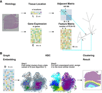
The workflow of clustering analysis using KBC. (A) Beginning with a spatial transcriptomics (ST) data set, the spatial information L and the gene expression information E are integrated to produce a graph that contains both cell location and gene expression information. (B) A graph-embedding scheme converts a graph into a vector representation, as shown on the left, which is ready to be used for clustering. The illustration shows the two steps of the proposed KBC algorithm.
As the focus of this paper is clustering, we highlight the distinctive features of KBC in comparison with existing clustering algorithms such as k-means (MacQueen 1967) and Louvain (Blondel et al. 2008). The first distinct feature of KBC has two key aspects. First, KBC treats points in a cluster as independent and identically distributed (iid) samples from an unknown distribution. Second, KBC employs a distributional kernel to represent and grow a cluster. The first aspect forms the foundation of the entire algorithm, whereas the second aspect is encapsulated in the second step of KBC. Although some existing clustering algorithms such as density-based methods and Gaussian mixture models (GMMs) have considered clusters as distributions, they must employ either a density estimator or a mixture model to estimate the distribution. This is the source of the estimation error and high time complexity. KBC employs neither of them but a distributional kernel that does not need to estimate the distributions at all.
The first step of KBC is to identify k initial clusters, in which each cluster is treated as generated from an unknown distribution. They are discovered from a subset of the (embedded) data set D. The second step of KBC assigns each unassigned point in D to the most similar distribution (estimated from the points in an initial cluster), based on a distributional kernel. This gives rise to the first distinctive feature of KBC, namely, KBC discovers clusters of arbitrary shapes, sizes and densities, which are congruous to the distributions of the clusters in D. The details of the procedure are given in Algorithm 1 in the Methods.
Existing clustering algorithms have limitations in their ability to detect certain types of clusters. The limitation of k-means clustering is well studied; that is, it can only find clusters of globular shapes because each cluster is represented with an average vector (Aggarwal 2015). Although density-based methods (Ester et al. 1996; Rodriguez and Laio 2014) can detect arbitrary-shaped clusters, they have difficulties discovering clusters of varied densities (Zhu et al. 2016) and clusters of uniform distribution (in which a density estimator often produces multiple peaks in a cluster of uniform distribution, owing to estimation errors) (Zhu et al. 2022). Louvain, a commonly used clustering algorithm in ST, has similar issues because it is also based on density. Louvain is a community detection method that aims to find communities (i.e., clusters) in a network or graph. It maximizes modularity, which is a measure of the relative density of edges within each community compared with the density of edges between communities. The density of edges within a community is defined as the sum of edge weights between nodes that belong to the community. A recent study (Traag et al. 2019) shows that Louvain can produce arbitrarily badly connected clusters (or communities in a graph). Clustering based on GMM (Dempster et al. 1977; Traag et al. 1996) assumes that each cluster is a mixture of Gaussian distributions. This requires modeling the parameters of the Gaussian distributions and the weights of their mixtures, and accurate estimations often require a substantial amount of data. However, many ST data sets may not have sufficient data for GMMs to perform accurate estimations (Lyu et al. 2021). As a result, this often leads to suboptimal clustering outcomes. Mclust (Scrucca et al. 2016) is a typical GMM-based clustering algorithm used in the literature on ST (Zhao et al. 2021; Dong and Zhang 2022). Walktrap (Pons and Latapy 2005) relies on random walks in a network in order to identify communities in the network. The intuition is that random walks on a network tend to get “trapped” into specific communities, characterized by densely interconnected nodes, whereas the connections between different communities tend to be sparse. Walktrap defines a distance by using the properties of random walks (Aggarwal 2015) and then uses an agglomerative hierarchical clustering (AHC) algorithm based on Ward's method (Ward 1963) to perform the final clustering. As AHC is known to be sensitive to the merging criterion employed and unable to discover clusters of varied densities (Han et al. 2022), Walktrap has the same issue as other AHC-based clustering algorithms. In essence, none of the existing clustering algorithms are able to discover clusters of arbitrary shapes, sizes, and densities, and these kind of clusters often exists in ST data sets.
The second distinctive feature of KBC is that it is the first linear time-and-space-complexity clustering algorithm. None of the existing clustering algorithms have this feature. Even the fastest k-means has superpolynomial time complexity (Arthur and Vassilvitskii 2006), although it often exhibits linear time in small data sets. All the other clustering algorithms mentioned above have at least quadratic time complexity.
In addition, we introduce the WL graph embedding (Weisfeiler and Lehman 1968; Shervashidze et al. 2011; Togninalli et al. 2019) in the treatment of ST data for the first time. It has been theoretically proved that graph neural networks (GNNs) cannot be more powerful than WL in terms of distinguishing nonisomorphic (sub)graphs (Morris et al. 2019). This result holds for a wide range of GNN architectures and all possible parameter choices for them. Moreover, a straightforward and efficient implementation of WL is available (Xu et al. 2021), offering computational advantages and running orders of magnitude faster than existing GNN-based methods. Specifically, we demonstrate that WL produces clustering outcomes nearly as effective as SpatialPCA (Shang and Zhou 2022), the leading data transformation method in ST, while executing much faster.
Ablation studies
We aim to ascertain the importance of the two components in clustering ST data, namely, data transformation and clustering. To achieve this aim, we conduct two experiments to assess:
-
The relative performance of different data transformation methods, while performing the clustering with the same k-means clustering algorithm. The six methods under assessment are WL (Togninalli et al. 2019), SpatialPCA (Shang and Zhou 2022), Stagate (Dong and Zhang 2022), SpaGCN (Hu et al. 2021), stLearn (Pham et al. 2023), and PCA (Maćkiewicz and Ratajczak 1993).
-
The relative performance of different clustering algorithms, while using the same best data transformation method determined in the first experiment. The seven clustering algorithms under investigated are the proposed KBC, Walktrap (Pons and Latapy 2005), Mclust (Scrucca et al. 2016), k-means (MacQueen 1967), SpaGCN (Hu et al. 2021), BayesSpace (Zhao et al. 2021), and Louvain (Blondel et al. 2008).
The performance is assessed in terms of (1) the clustering outcome measured in adjusted Rand index (ARI) (Yeung and Ruzzo 2001) and normalized mutual information (NMI) (Cover 1999) and (2) the runtime on the same machine with an Intel i7-12700k and a NVIDIA RTX 3090 graphics card. We report the average ARI or NMI over 10 trials on each data set, as each of these methods has some form of randomization in the procedure. The LIBD human dorsolateral prefrontal cortex (DLPFC) (Maynard et al. 2021) data set, which is available at spatialLIBD and consists of 12 slices, is used in both experiments.
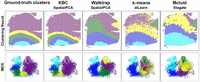
Figure 2 shows the results of the first ablation study. SpatialPCA yields the best clustering performance as shown in both violin plots of ARI and NMI, but it is the slowest compared with the other methods. SpatialPCA builds upon the probabilistic PCA, incorporates localization information as additional input, and uses a kernel matrix to explicitly model the spatial correlation structure across tissue locations. SpatialPCA uses SPARK (Sun et al. 2020) or SPARK-X (Zhu et al. 2021), depending on the size of the data set, to select the spatially variable genes (SVGs). In many slices, it learns the best feature representation. PCA, which is a cut-down version of SpatialPCA without the spatial information, produces the worst ARI/NMI result, but it is the fastest. This is not surprising because the spatial information is not used. WL, stLearn, and Stagate are the second-best methods with comparable ARI/NMI results, but WL runs at least one order of magnitude faster than the other two, even though WL uses the CPU and the other two utilize the GPU. In addition, WL runs three orders of magnitude faster than SpatialPCA. Stagate constructs a spatial neighbor network (SNN) based on the relative spatial locations of spots. Then, Stagate learns a low-dimensional embedding with spatial information and gene expressions via a graph attention auto-encoder. It can be observed that Stagate's embedding is not very good on this data set in Figure 2, A and B. The use of auto-encoder provides no advantage because it is computationally expensive and sensitive to parameter settings. stLearn employs a spatial morphological gene expression (SME) normalization method to learn an embedding. Out of all methods under comparison, stLearn is the only method that exploits all three types of information made available in spatially resolved transcriptomics (SRT), namely, spatial location, tissue morphology, and gene expression measurements. Yet, stLearn is not as effective as SpatialPCA and is only as good as WL. SpaGCN is the second-worst performer in terms of ARI/NMI, and it has comparable runtime (in the same order) with stLearn and Stagate. After calculating adjacent matrix, SpaGCN utilizes a graph convolution layer to aggregate gene expressions from neighboring spots. Note that GCN can use two layers only in practice, because using more layers can even hurt its performance (Zhang et al. 2019a). A recent study (Zhang et al. 2019b) shows that clustering can achieve good results without the use of graph convolution. Another interesting thing is that WL has been proven to be the best achievable by a GNN (Morris et al. 2019).
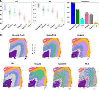
First ablation study. Comparing different data transformation methods using the same k-means clustering. (A) The violin plots show the ARI and NMI results of all 12 slices of DLPFC. The runtimes are shown in a bar chart. (B) The detailed clustering results of different embedding methods together with the ground-truth labels are shown for the slice 151673. Here, SpatialPCA, WL, and PCA ran on CPU only. Other methods ran on GPU.
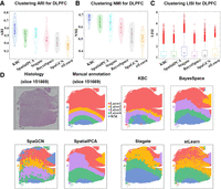
Figure 3, A and B, shows the results of the second ablation study, comparing seven clustering algorithms (using SpatialPCA as the data transformation method). The violin plot reveals that KBC is the best performer in terms of ARI and NMI. Walktrap, Mclust, and k-means are the second-best clustering algorithms having comparable result. SpaGCN and BayesSpace fall into the next tier, whereas Louvain is the worst performer.
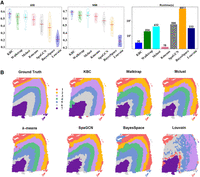
Second ablation study. Comparing different clustering algorithms using the same SpatialPCA embedding. (A) The violin plots show the ARI and NMI results of all 12 slices of DLPFC of the seven clustering algorithms. The runtimes are showed in a bar chart. (B) The detailed clustering results of different clustering methods are shown for the slice 151673. Only SpaGCN ran on GPU; others ran on CPU.
SpaGCN uses either Louvain or k-means to produce a set of initial clusters. As the final clustering outcome of SpaGCN heavily relies on the quality of the initial clusters, when they do not represent the clusters well, they often lead to poor final clustering outcomes. The issues with Louvain and k-means have been presented in the section Method Overview.
BayesSpace is a Bayesian statistical method that encourages neighboring spots to belong to the same cluster by introducing a spatial prior into the spatial neighborhood structure. BayesSpace performs the Bayesian clustering after obtaining initial clusters using either k-means or Mclust. If ground-truth clusters overlap, which often occurs in ST data, k-means or Mclust will produce poor (initial) clusters, leading to the poor final clustering of BayesSpace.
The fastest clustering algorithms are k-means and KBC; their runtimes are in the same order of magnitude. Walktrap, Mclust, SpaGCN, and Louvain are the second fastest, but they are one order of magnitude slower than k-means and KBC. BayesSpace is the slowest, which is two orders of magnitude slower than k-means and KBC.
Summary of the two ablation studies
In a nutshell, the two components (i.e., data transformation and clustering) are equally important. Although significant advancements have been made in data transformation, clustering algorithms remain a less researched area in the ST domain. As articulated in the Introduction, all known works have utilized existing clustering algorithms.
Although SpatialPCA is the best data transformation method in our study, it is the slowest. Its contender is the proposed WL scheme, which has slightly weaker embedding outcome but runs three orders of magnitude faster. Note that the relative clustering outcome between SpatialPCA and WL is on this particular data set only. We will see later that the outcome is reversed on other data sets.
Among all clustering algorithms examined, the proposed clustering KBC is a clear winner in terms of both clustering outcome and runtime.
The ability to find clusters of varied densities and overlapping clusters
Here we examine the ability of a clustering algorithm to find clusters of arbitrary shapes, sizes, and densities using simple two-dimensional data sets, without the need to use a data transformation method. The data sets are those used previously to investigate the fundamental problems of spectral clustering (Nadler and Galun 2006). The first (3Gaussians) data set, shown in Figure 4C, is composed of one sparse Gaussian distribution and two dense Gaussian distributions, having 300 points per cluster. The second (StripC) data set, shown in Figure 4D, comprises a thin strip cluster and a circle with 700 points per cluster. The first examines the ability of a clustering algorithm to separate clusters of varied densities; the second assesses the ability to separate two overlapping clusters. Note that these are not data sets trying to simulate the characteristic of ST data. They are designed to reveal an algorithm's fundamental clustering limitations if it could not successfully cluster these simple data sets.
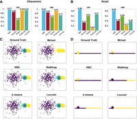
Examining the ability to find clusters of varied densities and overlapping clusters on two synthetic data sets: 3Gaussians and StripC. (A) The bar charts (in terms of ARI and NMI) of the five clustering methods on 3Gaussians. (B) The bar charts of the five clustering methods on StripC. (C) The ground truth and the clustering results of the five clustering methods on 3Gaussians. (D) The ground truth and the clustering results of the five clustering methods on StripC.
The clustering outcomes of five clustering algorithms are shown in Figure 4, A and B. On the 3Gaussians data set, KBC is the best performer, having ARI = 0.97, matching almost perfectly with the ground-truth clusters. Louvain, Waltrap, and k-means are the second-best performers as they have overextended the middle dense cluster to include neighboring points of the sparse cluster. Mclust has the same issue but with an additional shortcoming; namely, the two dense clusters have been merged into one. It is the only clustering algorithm that made this mistake.
On the StripC data set, KBC also has the best result with ARI = 0.88, which best matches the ground-truth clusters. Louvain, Walktrap, and k-means have the same handicap; that is, each separates the thin strip cluster into two halves, although at different locations on the strip cluster. Mclust has done the reverse; namely, it identifies correctly the strip cluster but includes parts of circle to be members of the strip cluster.
These poor clustering outcomes of the existing clustering algorithms are reminiscent to those of spectral clustering, having fundamental limitations identified previously (Nadler and Galun 2006). In short, these clustering algorithms have the fundamental limitations to discover clusters of arbitrary shapes, sizes, and densities.
KBC successfully discovers clusters of arbitrary shapes, sizes, and densities on an ST data set, but others fail
In addition to the clustering capability of KBC shown thus far, we demonstrate here the ability of KBC to find clusters of arbitrary shapes, sizes, and densities on an ST data set, whereas others fail to do so.
Figure 5 compares the clustering outcomes of four clustering algorithms on the DLPFC data set. The density contour map, shown in the second row (which is the same for all plots), provides interesting information. First, there are two large clusters on either side of a deep density valley in the middle. In the ground-truth column, the right (purple) cluster has one clear density peak, and the left (blue and green) cluster has two clear density peaks, where the former is much denser than the latter. The light blue and yellow regions are the lowest-density regions (outside the white region, which has no data).
Clustering outcomes on the density contour map created using multidimensional scaling (MDS) (Torgerson 1952). MDS reduces the number of dimensions of the features derived from SpatialPCA (identified to be the best data transformation method previously). The density is estimated using kernel density estimation (Scott 2015) on the space of the MDS reduced dimensions. The data transformation methods used are SpatialPCA, stLearn, and Stagate, and the clustering methods are as employed in their respective papers (Dong and Zhang 2022; Shang and Zhou 2022; Pham et al. 2023), except the proposed KBC.
There are three interesting observations:
-
KBC is the only clustering algorithm that can correctly identify the densest purple cluster as one single cluster. All the other algorithms split this cluster into multiple smaller clusters.
-
KBC also correctly splits the second densest two-peak cluster into two. SpatialPCA (with Walktrap) and stLearn (k-means) identify it as one cluster only.
-
KBC correctly identifies the region in-between the two densest clusters as a single low-density (yellow) cluster and as another low-density (light-blue) cluster at the edge of the dense (blue) cluster. Although Walktrap (with SpatialPCA) and k-means (with stLearn) can also correctly identify the light-blue cluster, they did poorly on the second-densest cluster and the low-density region in-between the two densest clusters. Mclust (with Stagate) is the worst performer in these regions, in which each of these low-density regions is merged with a neighboring dense cluster.
KBC is a linear time-and-space-complexity clustering algorithm
The time complexities of KBC and k-means (Hartigan and Wong 1979) are O(n), where n is the data set size. Other clustering algorithms such as Mclust (Scrucca et al. 2016), SpaGCN (Hu et al. 2021), and BayesSpace (Zhao et al. 2021) have O(n2) time complexity; Louvain has O(nlog(n)) (Blondel et al. 2008); and Walktrap (Pons and Latapy 2005) has O(n2log(n)). The algorithms with at least quadratic time complexity are unable to deal with large-scale data sets.
We conduct a scaleup test to examine the scalability of seven clustering algorithms. The results of the scaleup test on the seven clustering algorithms are shown in Figure 6. In terms of runtime, BayesSpace is the slowest which, is four orders of magnitude slower than the fastest KBC and k-means at data size 104.5. The other four clustering is at least two orders of magnitude slower. The gap is getting worse as the data size increases (except Mclust). In terms of runtime ratio, KBC and k-means have linear time, and all other methods (except Mclust) have at least quadratic time. Note that SpaGCN ran on GPU, and other methods ran on CPU. Yet, SpaGCN still ran significantly slower than KBC and k-means.
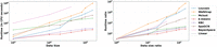
Scaleup test result for different clustering algorithms on the Slide-seq V2 mouse hippocampus data set (Stickels et al. 2021). This data set facilitates the creation of increasing larger subsets for the test. The data sizes range from 1000 to 160,000. We reduce the dimensionality of the data set using principal component analysis (PCA) and retain the top 20 principal components, which capture the majority of the variance in the data set. This is used for all algorithms. The data set size has 1000 points at data size ratio = 1. BayesSpace has no results on larger data sets because it took >48 h. Note that SpatialPCA and stLearn employ Walktrap and k-means/Louvain, respectively, as their clustering algorithms. Only SpaGCN's runtime is in GPU seconds. Note that the linear time has a gradient of one in the runtime ratio plot (shown by the line labeled as linear). Those runtimes that are worse than linear have a higher gradient.
These results are consistent with the time complexities of the algorithms shown earlier. There are two exceptions. First, Mclust runs in linear time, instead of quadratic time stated in the original paper (Scrucca et al. 2016). An examination of the code indicates that the speedup could be caused by the use of a kind of search (default hard coded setting), which limits to a fixed number of models examined in order to reduce the runtime. Second, Louvain runs significantly slower than O(nlog(n)), and we suspect that the time complexity stated in their paper is incorrect.
The space complexities of KBC and k-means are O(n), and the space complexity of Walktrap is O(n2). The space complexities of Mclust, Louvain, BayesSpace, and SpaGCN are not specified in their papers.
We have used the names of the existing methods to refer to the data transformation methods only thus far. In the rest of this paper, the name of each existing method refers to both the data transformation method and the clustering algorithm employed in their individual paper. KBC uses the WL embedding in the following sections.
Application of KBC to the HER2 tumor data
The overexpression of ERBB2 (also known as human epidermal growth factor receptor 2 [HER2]) on tumor cells defines the major subtypes of breast cancer. HER2-positive tumors are typically caused by the amplification of a domain on Chromosome 17 (cytogenetic band Chr17q12) containing the ERBB2 gene.
The source of HER2-positive breast tumor data collected from the ST platform (Andersson et al. 2021) has a data set containing 36 samples, labeled from patient A to patient H, each of which has different numbers of sections. Following the method of Shang and Zhou (2022), we have selected eight patient sections (A1–H1) as our experimental data for clustering analysis. Figure 7, A–C, shows the overall results obtained from different methods.
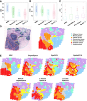
Application of KBC to the HER2 tumor data. (A,B) The violin plots of results obtained from different methods (for sections A1 to H1). (C) The boxplot in terms of local inverse Simpsons index (LISI) (Korsunsky et al. 2019) for different sections (from A1 to H1). A lower LISI value indicates a more uniform cluster of adjacent spatial domains. Thus, the smaller LISI the better. The red cross points are outliers of the LISI. (D) The histology image and manual annotation plot of section H1. (E) Clustering outcomes of four methods: KBC, BayesSpace (k-means), SpaGCN (Louvain), and SpatialPCA for section H1. The bottom row indicates three example cluster outcomes of BayesSpace and SpaGCN, but they employ the initial clusters produced by Mclust, k-means, and Louvain, respectively. Two results of SpaGCN use Louvain to produce the initial clusters but with different parameter settings.
Following the method of Shang and Zhou (2022), we show the detailed results of section H1 in Figure 7, D and E. This particular section includes approximately 10,000 genes and 600 cells collected from ST. The HER2 tumor data set has been examined and annotated by a pathologist, resulting in seven spatial domains in section H1, as shown in Figure 7D. The focus is on two domains: The orange domain corresponds to cancer in situ, and the red domain corresponds to invasive cancer. The connective tissue has the most cells and overlaps with five other domains. The domain annotation has provided us with a valuable reference that we can use to evaluate the effectiveness of each clustering outcome.
The HER2 tumor data set is more challenging than the DLPFC data set (used before this section) in a clustering task for two reasons. First, the size of the HER2 tumor data set is small. As a result, the data quality may not be high enough. Second, the spatial structure of the HER2 tumor data set is more complex than that in the DLPFC data set. As seen from Figure 7D, each domain has more than one cluster; for example, invasive cancer has two clusters, and cancer in situ has three clusters. In contrast, the DLPFC data set has only one contiguous cluster for each type (see the ground truth in Fig. 2B). The clustering outcomes on this data set, presented thus far in the current literature, are not satisfactory. This is consistent with our repeated experiment using their methods (see our result below).
Our experimental result shown in Figure 7E reveals that KBC successfully identified the two cancer domains, namely, cancer in situ and invasive cancer. In this task, it is crucial to detect and distinguish these two cancer domains.
Yet, all other methods can only partially detect some subdomains, and they are often fragmented. For example, although SpatialPCA has identified the two cancers, there are many incorrect identifications; for example, a large noncancerous domain was identified as cancerous, and cancer in situ was mistaken as invasive cancer, and vice versa. In addition, the two cancers identified are fragmented, and the regions of the correct identifications are small.
This poor clustering outcome of SpatialPCA has two main reasons. First, it is the use of the Walktrap clustering algorithm, in which its weakness has been stipulated in the ablation study section. Second, the spatial information learning ability of SpatialPCA is not suitable for the spatial structure of this data set. We have applied KBC on the SpatialPCA transformed data but still could not get good results. This is one of the example data sets for which SpatialPCA is not the best data transformation method, unlike what we have shown earlier using the DLPFC data set.
The weak clustering outcomes of BayesSpace and SpaGCN may be owing to the clustering algorithms employed to perform the initial clustering. They use k-means, Louvain, or Mclust to find the initial clusters. As can be seen in the last row in Figure 7E, the clustering results of k-means, Louvain, and Mclust are not good enough. Using them as the initial clusters is not a good choice. In addition, excluding the impact of initial clusters employed, the clustering performances of SpaGCN and BayesSpace are not good either. For example, SpaGCN does not produce a clustering result that is better than its initial clusters, produced by Louvain.
The clustering result of KBC was the best because almost every cluster discovered has a solid mass of neighboring points, and many clusters correspond closely to the annotated domains. This is also reflected in terms of ARI and NMI results, which are the highest among all contenders (Fig. 7A,B). Also, KBC's median LISI = 1.28 is also the best (the median LISIs of SpatialPCA, BayesSpace, and SpaGCN are 1.84, 1.74, and 2.13, respectively) (Fig. 7C).
Clustering plays an important role for discovering new biological insights from spatial genomics data. Here we provide an example. There are two key discrepancies between the ground-truth labels and the clusters identified by KBC. First, KBC suggests that the cells in bottom-left region are from the same group, but the ground-truth labels indicate that it has two separate regions of invasive cancer and cancer in situ. Second, the middle-right region is identified to be immune infiltrate by KBC, but the ground truth label is breast glands. Our examination via differential expression analyses reveal that some ground-truth labels may be re-examined (for details, see Supplemental Fig. S1 in Supplemental Text S2, Further Analysis of the KBC Clustering Outcomes of the HER2 Tumor Data). It is important to note that ground-truth labels are often assigned by humans, who may introduce potential errors in the labeling process.
Application of KBC to the mouse hippocampus data
We downloaded the Slide-seq V2 (Stickels et al. 2021) data set from the Single Cell Portal SCP815 website and focused on the mouse hippocampus data (in the file named “Puck_200115_08”). The sample contains 53,208 cells, each having 23,264 genes. To have a fair comparison of all methods, any data transformation method employed deals with the same gene expression and spatial information. This data set does not have tissue domain annotation that could be used as ground truth. So, we relied on the Allen Brain Atlas (Fig. 8A) to help us understand the original tissue structure. Note that although the Allen Brain Atlas provides the regional divisions, there are no good mappings between the altas and the data set, so it cannot be relied upon completely.
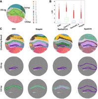
Application of KBC to the mouse hippocampus data. (A) Allen Brain Atlas P56 coronal. The diagram shows the structure of the mouse hippocampus. (B) The LISI index of the clustering results of KBC, SpaGCN, SpatialPCA, and Stagate. (C) A comparison of four clustering results on the CA1sp domain and the DG-sg domain.
The spatial domains identified by KBC, SpatialPCA, and Stagate were consistent with the coronal mouse olfactory bulb from the Allen Brain Atlas in the central area, labeled as CA1sp and CA3sp in Figure 8A. Looking at the CA1sp, CA3sp, and DG-sg domains only in Figure 8C, all methods could identify these domains. The exception is SpaGCN, which groups all three domains into one single cluster. KBC's clustering outcome, shown in Figure 8C, matches the most to the Allen Brain Atlas, in which each of the three domains is accurately identified. In terms of identifying the DG-sg domain, KBC and SpatialPCA produce similarly good results, but Stagate's result is not satisfactory because the cluster merges with other domains. In addition, KBC clearly distinguishes the CA1sp domain from the other domains. But, SpatialPCA produces a cluster that encompasses more than the CA1sp domain. For the CA3sp domain, the results of the KBC, Stagate, and SpatialPCA are similar.
In terms of LISI, KBC has the smoothest clustering result, achieving the lowest mean LISI = 1.03 among all the four methods shown in Figure 8B. Note that no ARI/NMI results can be produced because there is no ground truth in this data set.
This data set is the largest of the data sets used in this paper, almost one order of magnitude larger than the DLPFC data. Therefore, the clustering of this data set took significantly more computing resources than other data sets. Yet, the proposed KBC and graph-embedding WL could complete running this data set in a short time. The WL graph-embedding method took 2541 sec, which is the fastest. In comparison, the other methods took >10,000 sec. For the clustering component, KBC took 5 CPU seconds, whereas the fastest of the other methods, SpaGCN, took 231 GPU seconds.
Application of KBC to the DLPFC data
DLPFC (Pardo et al. 2022) is a 10x Genomics Visium data set generated from healthy human brain samples from the DLPFC domain. We downloaded the data set from the spatialLIBD website. There are 12 samples from three individuals in the full data set. Each sample has been manually annotated with the white matter (WM) and layers of the cortex based on the morphological features and gene markers (Maynard et al. 2021). These annotations are treated as ground-truth labels.
Here we take DLPFC tissue slice 151669 as an example to demonstrate the advantages of KBC. The tissue slice has 3661 spots and 33,538 genes. The spots are divided into five groups with four layers and the WM. The manual annotation plot in Figure 9D shows the distribution of these five groups, which have distinctive layers from top to bottom. Layer1 is the largest, which has 2141 cells, whereas others have only 400 cells on average. It can be clearly seen from Figure 9D that KBC has achieved the best result in terms of recognizing the largest (red) domain of Layer1. Other methods tend to divide Layer1 into several clusters. For all 12 slices, KBC achieves the highest accuracy with a mean ARI 0.58 (Fig. 9A) and a mean NMI 0.68 (Fig. 9B). In terms of LISI, KBC produces the lowest mean LISI = 1.06 (Fig. 9C).
Application of KBC to the DLPFC data. (A,B) The violin plots of the results obtained from six different methods on the DLPFC data set. (C) The boxplot of clustering LISI of the six different methods on the DLPFC data set. (D) Histology image, manual annotation (Maynard et al. 2021), and the clustering results of KBC, BayesSpace, SpaGCN, SpatialPCA, Stagate, and stLearn plotted on DLPFC slice 151669.
Studies on simulated ST data
SRTsim, which is developed by Zhu et al. (2023), is a spatial pattern preserving simulator for scalable, reproducible, and realistic SRT simulations. Here we apply SRTsim to generate simulated data sets. The LIBD human DLPFC (Maynard et al. 2021) data set (12 sections from 151507 to 151676) are used as references for SRTsim to conduct reference-based tissue-wise model fitting and data simulation procedures. Specifically, we randomly generated a simulated data set for each section of the real data. We further selected up to 3000 significant SVGs with SPARK (Sun et al. 2020) and the top 2000 highly variable genes (HVGs) with Seurat (Satija et al. 2015) for each simulated section to generate the SVG and HVG data sets for each section. To demonstrate the robustness of the proposed method, we conducted the experiments 10 times with different random seeds and evaluated the performance of each method on each of the simulated SVG and HVG data sets.
Based on the simulated data sets, we conducted ablation studies to investigate the clustering performance of different clustering algorithms, including KBC, Walktrap, k-means, and Mclust, as well as different embedding methods, such as WL and SpatialPCA. Additionally, we performed sensitivity analyses focusing on the number of principal components used in the data preprocessing steps (Supplemental Fig. S2), the parameters ψ and τ chosen for KBC (Supplemental Fig. S3), and the parameter h in WL (Supplemental Fig. S4). The detailed results are presented in the following subsections. Parameter search ranges used in the experiments are shown in Supplemental Text S1 (Supplemental Table S1).
Ablation studies on simulated data sets
This section reports the results of ablation studies on simulated data sets to evaluate the performance of different clustering algorithms (KBC, Walktrap, k-means, and Mclust) and embedding methods (WL and SpatialPCA). They are the best clustering algorithms and data transformation methods found in the two ablation studies we have reported in the section on ablation studies. The experiments are conducted on both simulated HVG and SVG data sets.
When integrated with the same embedding method (either WL or SpatialPCA), KBC clearly outperforms other algorithms in either setting, achieving the highest median NMI and ARI scores (represented by hollow circles in Fig. 10). Furthermore, SpatialPCA + KBC outperforms WL + KBC in both HVG and SVG data sets. Note that these observations are consistent with the results presented in the section on ablation studies.
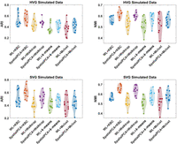
Results of the further ablation studies on four clustering methods and two data transformation methods using the HVG and SVG simulated data sets.
A caveat is in order with regard to SpatialPCA + KBC, which has the best performance on the DLPFC data set (as reported in the section on ablation studies) and on the simulated data sets based on the same DLPFC data set. One shall take care in generalizing this outcome to other data sets. As we have pointed out in the two sections on the HER2 tumor and mouse hippocampus data sets, the WL method works much better than SpatialPCA on these data sets, which contain complex patterns.
Discussion
WL and SpatialPCA are efficient methods for data transformation and dimension reduction. When integrated with WL or SpatialPCA, KBC can accurately identify spatial domains in a single tissue section. However, WL and SpatialPCA could not directly handle data from multiple batches or tissue sections. When analyzing multiple batches or tissue sections, our pipeline could either (1) analyze each tissue independently with WL or SpatialPCA or (2) use an alternative data transformation method that could correct batch effects and simultaneously integrate multiple sections. Recently, a dependency-aware deep generative model spaVAE has been proposed (Tian et al. 2024) that could jointly model multiple batches and sections by conditional variational auto-encoders and perform efficient dimension reduction for a SRT data. Equipped with the transformed data generated by spaVAE, KBC (or any stand-alone clustering method) is expected to detect cell types across related tissue sections concurrently.
We have only used data sets with non-single-cell resolution in our applications thus far. But, neither the WL/SpatialPCA method nor KBC is limited to this resolution only. These methods are natively applicable to data sets generated by ST technologies with cellular or subcellular resolutions. Supplemental Text S4 (Supplemental Fig. S8) shows an example result of KBC integrated with WL for analyzing the mouse olfactory bulb Stereo-seq data (Chen et al. 2022). Stereo-seq is a newly emerging ST technology that could achieve the cellular or subcellular spatial resolution by DNA nanoball patterned array chips (Chen et al. 2022). As shown in Supplemental Text S4, the results from KBC accurately reflected the laminar organization and corresponded well with the annotated layers.
Note that the above-mentioned two capabilities of KBC are the same for all clustering methods, independent of the data transformation employed and the SRT technology used.
Methods
Data preprocessing
For all data sets, we normalized the raw molecular count matrix using the variance stabilizing transformation method called SCTransform (Choudhary and Satija 2022), which is a negative binomial regression model implemented in the Seurat package (Satija et al. 2015). Following the method of Shang and Zhou (2022), we filter genes to reserve a set of SVGs only. Specifically, we apply SPARK (Sun et al. 2020) for SVG analysis in small data sets owing to its higher statistical power and use SPARK-X (Zhu et al. 2021) for SVG analysis in large data sets (e.g., the mouse hippocampus data set) in order to save time and memory. We select up to 3000 significant SVGs for each single data set with a false-discovery rate (FDR) of 0.05 as input. The normalization and gene selection steps are conducted with the default parameters recommended by those packages. The details of the original data source of each data set used and the sources of competing methods can be found in the Supplemental Text S1 (Supplemental Table S2).
The processed expression matrix is centered (to have zero mean) but not scaled for each feature before applying the principal component analysis (PCA). Here, we applied PCA to extract the first 15 principal components to produce the feature matrix to represent the gene expression. We show in Supplemental Figure S2 (in Supplemental Text S2) that the proposed pipeline is robust against the number of principal components selected. At the end of the preprocessing, a gene expression feature matrix of m (genes) × n (tissue locations) was obtained.
A k-nearest neighbor search was performed on the spatial coordinates. Depending on the SRT technology employed, there are four (k = 4) and six (k = 6) neighboring spots for ST platform (Andersson et al. 2021) and Visium (Pardo et al. 2022), respectively. An adjacency matrix was generated based on the locations of neighboring cells. Note that this is the data characteristic, and this property is used for all methods of data transformation, including the WL method we introduced.
The combined information from the gene expression feature matrix and the adjacency matrix produces a graph. Then, a graph-embedding method (Supplemental Table S3), such as the WL scheme, converts the graph to an embedded matrix of h × n, where h is the parameter of the WL scheme. Note that many data transformation methods, such as Stagate and SpaGCN, also involve a graph and thus require graph embedding, albeit the actual embedding methods employed differ. A clustering algorithm such as the proposed KBC takes the embedded matrix as input to find the clusters in it.
Kernel bounded clustering
Let  be a kernel that measures the similarity between two points
  , and let
  be a distributional kernel that measures the similarity between two distributions
  and
and  , where
  is an unknown distribution that generates iid points in set W ⊂ ℝd. Further let
  be a Dirac measure that converts a point x into a distribution.
Given a data set D ⊂ ℝd, the proposed clustering algorithm, named kernel-bounded clustering (KBC), discovers the clusters in D. KBC has two key steps, as shown in Algorithm 1. The first step identifies k initial clusters Gj having points with similarities higher than a threshold τ. As points in each of the initial clusters have high similarity to each other, they are good representatives of a distribution that generates these points. As a result, the initial clusters can be obtained using a subset of the given data set, namely, Ds ⊂ D, in order to reduce its time complexity.
Kernel bounded clustering
input: D- given data set, k- number of clusters, s- sample size, τ- similarity threshold
output: ℂ = {C1, …, Ck}
1. From Ds ⊂ D, find the largest k initial clusters Gj via kernel κ as follows: 
 .
.
2. From D, recruit members of Ci via distributional kernel K and initial clusters Gj, j = 1, …, k:

 .
.
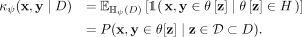
The second step recruits members of each cluster from D via a distributional kernel K by assigning each point  to a distribution estimated by initial cluster G in which x has the highest similarity, as measured by K.
Using kernel mean embedding (Smola et al. 2007; Muandet et al. 2017), the empirical estimation of the distributional kernel K on two distributions  and
and  , which is based on a point kernel κ on points
  , is given as
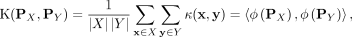 (1)
where
(1)
where 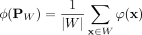 is the empirical estimation of the feature map of
  , and
, and  is the feature map of the point kernel
  .
.
The distributional approach for clustering has two main advantages over a nondistributional approach. First, the discovered clusters can have arbitrary shapes, varied sizes and densities. This is because each cluster is represented as a distribution, and using a nonparametric method such as kernel mean embedding, the distribution does not need to be modeled and it can be left unknown. Second, the kernel computation is very efficient using a finite-dimensional feature map of the kernel (for details, see Ting et al. 2020; Xu et al. 2021). KBC has linear time complexity O(s2 + kn), as all parameters, except n, are constant.
KBC employs isolation kernel
The proposed KBC shall use isolation kernel, a data-dependent kernel introduced recently (Ting et al. 2018; Qin et al. 2019). It has been shown to improve the accuracy of SVM classifier and density-based clustering algorithm DBSCAN. The pertinent details of isolation kernel are provided in this section.
Let D ⊂ ℝd be a data set sampled from an unknown  , and let
  denote the set of all partitionings H that are admissible from
  , where each point
  has the equal probability of being selected from D, and
  Each isolating partition
  isolates a point
  from the rest of the points in D. Let 1( · ) be an indicator function.
For any two points  , the similarity of x and y, as measured by isolation kernel (Ting et al. 2018; Qin et al. 2019), is defined to be the expectation taken over the probability distribution on all partitionings
  that both x and y fall into the same isolating partition
  :
: (2)
(2)
In practice,  is constructed using a finite number of partitionings Hi, i = 1, …, t, where each Hi is created using a randomly sampled subset
  , and θ is a shorthand for
  :
: (3)
(3)
Isolation kernel defines a reproducing kernel Hilbert space because Equation 3 is a quadratic form.
The isolation partitioning mechanisms that have been used previously to implement isolation kernel are iForest (Liu et al. 2008; Ting et al. 2018), Voronoi diagram (Qin et al. 2019), and iNNE (Bandaragoda et al. 2018). We use iNNE in this work.
Each point  is isolated from the rest of the points in D by building a hypersphere that covers z only. The radius of the hypersphere
is determined by the distance between z and its nearest neighbor in D. In other words, a partitioning H consists of ψ hyperspheres
is isolated from the rest of the points in D by building a hypersphere that covers z only. The radius of the hypersphere
is determined by the distance between z and its nearest neighbor in D. In other words, a partitioning H consists of ψ hyperspheres  and the (ψ + 1)-th partition. The latter is the domain in ℝd, which is not covered by all ψ hyperspheres, where 2 ≤ ψ < |D|.
The feature map of isolation kernel. For point  , the feature mapping
  of
of  is a vector that represents the partitions in all the partitioning
  , i = 1, …, t, where x falls into either only one of the ψ hyperspheres or none in each partitioning Hi.
Let 1 denote the value of  such that
  and
and  for any j, k ∈ [1, ψ].
φ has the following geometrical interpretation:
-
 and
and  iff
iff  for all i ∈ [1, t].
-
For point x such that
 , then
-
If point
 falls outside of all hyperspheres in
  for all
  , then it is mapped to the origin of the feature space
  .
.
Note that the isolation kernel is a data-dependent kernel, which derives its feature map from a data set directly, and it has no closed form expression. In contrast, the Gaussian kernel, like most other commonly used kernel, is a data-independent kernel, which has a closed form expression. A comparison between the isolation kernel and Gaussian kernel and adaptive Gaussian kernel (Zelnik-Manor and Perona 2005) used in KBC can be found in Supplemental Text S3 (Supplemental Figs. S5–S7).
Software availability
The preprocessed spatial genomics data sets we used and the KBC software code are available at GitHub (https://github.com/IsolationKernel/Kernel-Bounded-Clustering-for-Spatial-Transcriptomics) and as Supplemental Code. The source code is released under a noncommercial use license.
Competing interest statement
The authors declare no competing interests.
Acknowledgments
K.M.T. is supported by the National Natural Science Foundation of China (NNSFC, grants no. 92470116 and no. 62076120). J.Z. is supported by the Natural Science Foundation of Jiangsu Province (grant no. BK20230781) and the NNSFC (grant no. 62306134).
Author contributions: KBC model development and implementation were by H.Z. Conceptualization and experimental design were by Y.Z., K.M.T., and J.Z. Experiments and data analysis were by Y.Z. and Q.Z. Supervising was by K.M.T. and J.Z. Writing was by Y.Z., K.M.T., and J.Z. All authors critically reviewed the manuscript.
Footnotes
-
[Supplemental material is available for this article.]
-
Article published online before print. Article, supplemental material, and publication date are at https://www.genome.org/cgi/doi/10.1101/gr.278983.124.
-
Freely available online through the Genome Research Open Access option.
- Received January 17, 2024.
- Accepted December 19, 2024.
This article, published in Genome Research, is available under a Creative Commons License (Attribution-NonCommercial 4.0 International), as described at http://creativecommons.org/licenses/by-nc/4.0/.


