
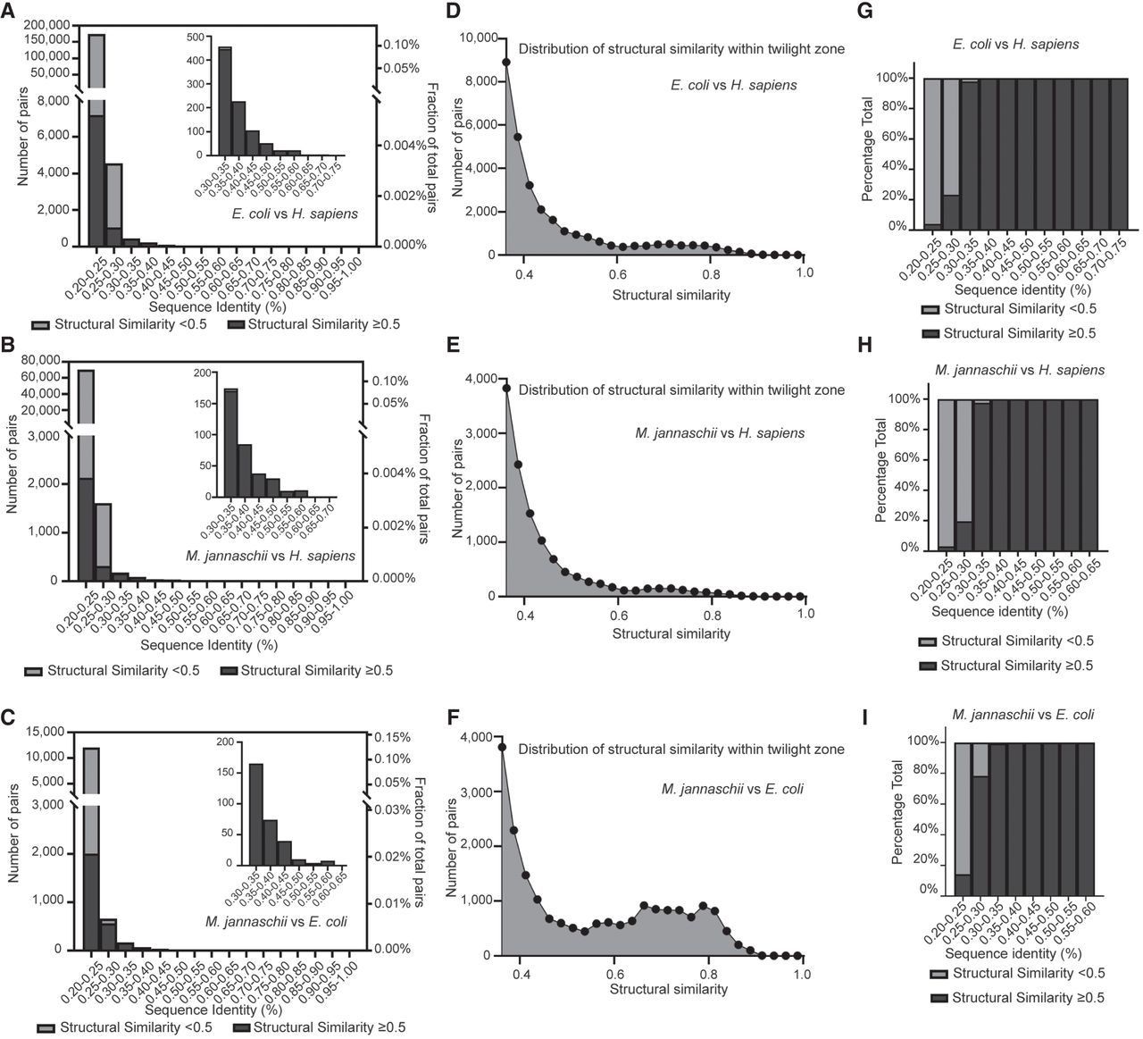
Examination of the distribution of structural similarity across different ranges of sequence identity. (A–C) Numbers of protein pairs (left, y-axis) and proportion in all possible combinations (right, y-axis) across different sequence identity ranges. The inserted pictures at the top right corner depict zoomed-in figures for protein pairs with sequence identity above 0.3. The subfigures compare the proteomes of E. coli versus H. sapiens (A), M. jannaschii versus H. sapiens (B), and M. jannaschii versus E. coli (C). The light gray color bar indicates those with structural similarity less than 0.5, and the dark gray color bar indicates those with structural similarity equal to or greater than 0.5. The light gray bar is invisible in the zoomed-in pictures at the corners, because very few protein pairs are identified with structural similarity less than 0.5 within the indicated ranges. (D–F) Distribution of structural similarity within the twilight zone, defined as sequence identity between 0.2 and 0.25. The subfigures compare the proteomes of E. coli versus H. sapiens (D), M. jannaschii versus H. sapiens (E), and M. jannaschii versus E. coli (F). The bin size for the distribution plot is 0.25. (G–I) The percentage fraction of protein pairs with structural similarity greater or less than 0.5 across different sequence identity ranges. The subfigures compare the proteomes of E. coli versus H. sapiens (G), M. jannaschii versus H. sapiens (H), and M. jannaschii versus E. coli (I). The x-axis ends at a sequence identity range of 0.55–0.70 because no protein pairs are identified above this value range.


