On the probability that a novel variant is a disease-causing mutation

One major goal of human genetics is to identify sequence variants that contribute to disease susceptibility for the purpose of developing treatment or preventive measures. At present, over 10,000 phenotypic loci have been mapped and shown to be related to the development of inherited diseases in humans (OMIM, http://www.ncbi.nlm.nih.gov/omim/). For many of these loci, genes have been cloned and databases of known or suspected mutations exist (HUGO, http://www.hugo-international.org). However, independent evidence of a mutation's involvement with disease may not exist. Evidence may be limited to finding the variant in a single patient and not in a group of healthy controls. In what we have termed a “mutation-detection experiment,” a clinical geneticist looks for such a pattern in order to identify variants that may be associated with disease.

In a typical mutation-detection experiment, a patient may present with a well-characterized genetic disorder without carrying any previously described mutations in the associated gene. At this point, the entire gene or region may be sequenced in an effort to identify variants unique to this patient. Each base sequenced is a separate, although not independent, test. The question that we address is how to compute a P-value for such a mutation hunt, logically accounting for multiple testing, keeping in mind that most bases are not polymorphic. In other words, we have calculated the probability of finding a neutral polymorphism in a patient and not in a group of healthy controls, taking into consideration the length of sequence examined. Our method can also be applied to a traditional case-control study, in which a variant is found at different frequencies in a group of patients and a group of controls. Here, we extend the classic case-control analysis to account for the multiple testing that is inherent in examining some length of sequence to ascertain variants of interest.

Although the steps leading to the final equations are quite technical, the actual computation of a P-value for a given mutation-detection experiment is very simple and can usually be performed on a scientific calculator. For the case-control adjustment, which is fairly complex, we present a simple approximation.

Methods

Theoretical background

Below, we examine three mutation-detection scenarios. In the first, the patient is heterozygous at a base that is monomorphic in a group of controls. In the second, the patient is homozygous, while all controls are either heterozygous or homozygous for the other allele. In the third, a variant is found at significantly different frequencies among cases and among controls. For each of the above, we calculate the probability of finding a neutral variant that follows such a pattern under two assumptions, no recombination and free recombination between adjacent bases. In the Supplemental material, we extend our method to consider an inbred patient who is homozygous for a potential disease-causing allele and compound heterozygosity found in a patient, but not in controls. All calculations are based on a population of constant size, with no selection and no recurrent or back mutation.

Under the above assumptions, the probability that the frequency of the newer (derived) allele at a polymorphic site is between x and x + dx is approximately (Cx)^-1dx, where C is half the mean time to fixation or loss of the new allele (Ewens 1974). C for any population can be estimated by integrating (Cx)^-1dx over to , setting the integral to 1.0 and solving for C. C can also be estimated as a hitting time problem using the usual diffusion approximation (Kimura and Ohta 1969). Both methods give nearly identical estimates of C. For humans, the effective population size (N) is ∼10,000, yielding C ≈ 10. Table 1 gives the expected fraction of neutral variants in several frequency ranges in the human population, using N = 10,000 and C = 10. Assuming a larger value for N, or a rapidly expanding population, results in a greater proportion of rare sites than listed in Table 1.

Heterozygous patient

The probability that a SNP with derived allele frequency x will be observed to be polymorphic in a sample size of j chromosomes is 1 - x^j - (1 - x)^j. Given that a SNP is polymorphic in a sample of j chromosomes, the probability, ϕ₁, that the derived allele has frequency between x and x + dx is ϕ₁ represents the Bayesian posterior estimate of the allele frequency, with prior (Cx)^-1dx and likelihood of observation 1 - x^j–(1 - x)^j (Ewens 1974). For j = 2, such as for variants identified in a single individual, ϕ₁ simplifies to 2(1 - x)dx.

Using ϕ₁, the probability that k control individuals are homozygous for the ancestral (older) allele at a polymorphic site given heterozygosity in a patient is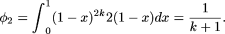

Probability of i mutations in a sequence of length L

The above are correct for a single segregating site. However, our major question of interest is how to account for the multiple testing that is inherent in querying some length of sequence in the patient for variants not found in controls. To do this, we model the distribution of the number of sequence variants expected within a single individual. Although estimating the expected number of segregating sites in a region is easy, the exact distribution is, in general, an unsolved problem for arbitrary levels of recombination. However, the distribution has been worked out under two extreme recombination scenarios, no recombination (Watterson 1975) and free recombination (Kimura 1969) between adjacent sites. Under no recombination, the distribution of the number of variant sites in a single diploid individual is approximately geometric. The probability of i variants in a sequence of length L bases is equal to 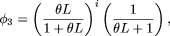where θ = 4Nμ. 4Nμ has been estimated at ∼8.25 × 10^-4 for the human genome as a whole (Halushka et al. 1999; Sachidanandam et al. 2001; Mitchell et al. 2004). Table 2 lists θ values for several different types of sequence (Cutler et al. 2001; Waterston et al. 2002; Thomas et al. 2003; Mitchell et al. 2004). Selecting the appropriate θ value for a given mutation detection experiment is covered in the Discussion section.

Using ϕ₂ and ϕ₃, the probability that the derived allele does not occur among k control individuals given heterozygosity in the patient, under a model of no recombination is

Technically, i is bounded above by L, but we have simplified the mathematics by ignoring this upper bound. This assumption does not appreciably change the outcome. Equation 2 contains two contradictory assumptions. The probability of i mutations was based on the assumption of no recombination, that is, complete linkage disequilibrium (LD). However, the probability of finding at least one neutral variant that is unique to the patient given i variants in the patient across the region assumes that all sites are independent of one another. This contradiction in terms can be resolved by modeling the distribution of the number of variable sites as Poisson(θL), which assumes free recombination (no LD) between adjacent sites. The probability of i segregating sites in a single diploid individual in the absence of LD, is therefore approximately [e^-θL(θL)ⁱ]/(i!).

Assuming free recombination between sites, the analogous computation to P₁ is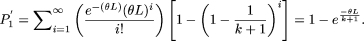

Homozygous patient, without inbreeding

For recessive diseases, we calculate the probability of finding a variant homozygous for the derived allele in the patient and either homozygous for the ancestral allele or heterozygous in controls. The derived allele frequency distribution, given homozygosity in the patient is 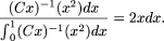The probability that k outbred individuals are not homozygous for the derived allele, given that the patient was homozygous is

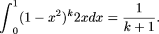
Because this value is identical to the probability of identifying a variant that is heterozygous in a patient and never seen in controls (equation 1), calculation of a P-value for a variant found homozygous in a patient and never in controls is identical to P₁ and P₁' under no recombination and free recombination, respectively. The equivalence can be explained intuitively in terms of combinatorics. If k is the number of control individuals screened, there are 2k + 2 chromosomes in total between the controls and the patient. When the patient is heterozygous and all controls are homozygous for the major allele, either of the two patient chromosomes could harbor the disease allele of the 2k + 2 total possible positions for the single copy of the minor allele. Thus, the probability that the variant is carried by the patient is (2)/(2k + 2), which reduces to (1)/(k + 1).

When the patient is homozygous for the derived allele and all other individuals are heterozygous or homozygous for the ancestral allele, there is one patient of k + 1 possible individuals, and the same result ensues.

Case-control study

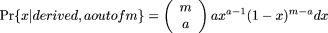
In case-control analyses, allele frequencies are compared between patients and controls. Alleles found at significantly different frequencies between the two groups are candidates for association with disease. We have developed a means to account for multiple testing in case-control studies, in which variants are identified by sequencing some or all of the cases. We have modeled an allele that has frequency a/m among cases and less than or equal to b/n among controls (a/m > b/n) or greater than or equal to b/n among controls (a/m < b/n).

The posterior distribution of the observed allele frequency (x), given that it appeared on a out of m chromosomes among the patients can be decomposed into the posterior allele frequency distribution of the observed allele, given that it is the derived allele and is observed on a out of m chromosomes, times the probability that we are observing the derived allele given a out of m plus the posterior allele frequency distribution of the observed allele, given that it is the ancestral allele and is observed on a out of m chromosomes, times the probability that we are observing the ancestral allele given a out of m. That is, The components of Pr{x| a out of m} are broken down below, with additional details in the Supplemental material. and Using Bayes' rule, 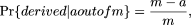and 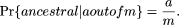The above represents the two-allele simplification of the classical infinite allele result (Watterson and Guess 1977). That is, in a finite population, the probability that a particular allele is the oldest is equal to its frequency.

Combining all of the components of the posterior distribution of the observed allele frequency, given that it appeared on a out of m chromosomes among the patients, yields

Incorporating information on allele frequency among the controls, the probability that the allele observed in a out of m case chromosomes will occur on exactly b out of n control chromosomes is 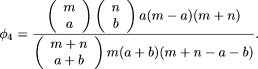If neutral allele has frequency a/m among patients, the probability that it has frequency less than or equal to k/n among controls is and the probability that it has frequency greater than or equal to j/n among controls is . So, the probability of finding a neutral allele at frequency a/m among cases and less than or equal to k/n or greater than or equal to j/n among controls is

Under a model of no recombination between sites, the explicit expression for the distribution of the number of segregating sites expected in a group of arbitrary size is complex and numerically unstable (Watterson 1975; Tavare 1984). Therefore, we have used Hudson's (1990) recursive formula. The probability of i segregating sites in a region of length L in a sample of m chromosomes is 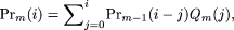where 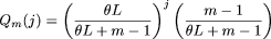and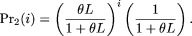

If L bases are resequenced among cases to identify variants, the probability that at least one identified site will have an allele with frequency less than or equal to k/n or greater than or equal to j/n among controls and frequency a/m among cases is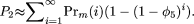

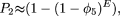
P₂ can be approximated by using the expected number of segregating sites in the region rather than the recursively defined distribution. where 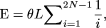the expected number of segregating sites in a region of length L in a sample of N individuals (Watterson 1975). If not all patient chromosomes were resequenced to identify new variants, E can be calculated using the number of patients that actually were screened.

Under free recombination, the number of segregating sites is assumed to be Poisson distributed with mean E. Thus,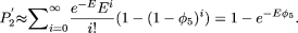

Simulations

To explore the effects of an expanding population on the probability of seeing a variant in a case and not in controls, we used coalescent theory to simulate a population with effective size 10,000 and current size 6 billion. Expansion from 10,000 to 6 billion took place in the population beginning 500 generations ago. The mutation rate was scaled down from 2.0625 × 10^-8 to 1.675 × 10^-8 mutations per base per generation for the expanding population simulations in order to generate the same expected number of segregating sites as were seen when the population size was assumed constant. 2.0625 × 10^-8 is the mutation rate that will lead to θ equal to 8.25 × 10^-4 for a population of size 10,000.

In addition, we modeled a population of constant size and verified that the probability of seeing a variant in a randomly chosen individual and not in any other individual was approximately the same as the value obtained using the mathematics presented earlier. All simulations were done assuming no recombination between sites.

Results

Table 3 gives the results, under our null neutral model, of no causal association between a variant and disease, for a mutation-detection experiment in which a single patient is heterozygous for a variant not found in a group of controls or for an experiment in which the patient is homozygous for a variant never found in homozygous state in controls. Table 3A contains three sections. In the first, the genome-wide average θ of 8.25 × 10^-4 is used. In the second and third sections, θ for coding regions, 4.8 × 10^-4, is used. The second section adjusts θ for a base that is conserved in mice, and the third adjusts θ for a base that is conserved in fugu. Within each section, the first column lists P-values associated with examining 10 kb of sequence in one patient and in 10–200 unaffected controls, and the second column gives the maximum length of sequence (kb) that may be examined to keep the P-value under 0.05. Table 3B compares P-values obtained using simulation for a population of constant size and for an expanding population. In Table 3B, the length of the region examined was held constant at 10 kb, and 10,000 replicates were performed to obtain each value. Table 3C gives the minimum size of the control group that must be examined in order to keep the P-value near 0.05 for 1–10 kb of sequence examined. The values in Table 3 were calculated using equation 2, which assumes no recombination between sites. Results for free recombination, obtained using equation 3, can be found in Supplemental Table 1 and Supplemental Figure 1.

Table 4A gives the P-values that would be obtained using our method for 5, 10, 20, and 50 kb examined and for a traditional case-control approach for varying allele frequencies with 50 cases and 50 controls, using equation 4. Table 4A also gives the expected number of polymorphic sites among a group of 50 individuals for regions that are 5, 10, 20, or 50 kb in length. In Table 4B, the length of sequence examined is held constant at 5 kb. P-values are shown for the traditional case-control method and for our method for case and control group sizes of 100, 200, and 500 individuals, assuming no recombination between sites. Analogous free recombination values obtained using equation 7 are given in Supplemental Table 2. Results for inbred homozygous patients and compound heterozygotes can be found in Supplemental Table 3 and Supplemental Figure 2, respectively.

Unless otherwise stated, all figures and tables wer egenerated using the genome-wide average θ, 8.25 × 10^-4, under the assumption of a constant population size, and completely neutral variation (no causal association of the variation with the disease).

Discussion

We have presented several methods for calculating P-values for mutation-detection experiments. These methods provide a solution to the multiple-testing problem that is inherent in such an experiment by taking into account the length of sequence examined for the purpose of identifying novel variants. Bases sequenced for this purpose are separate, although not independent, tests. By modeling the distribution of expected number of variants in a given region, we are able to account for the length of sequence examined in a biologically relevant manner.

Our method allows the selection of a θ value, the population mutation parameter, specific to a given experiment. We suggest several methods for estimating θ depending upon what is known about the sequence examined and the variant of interest. First, the genome-wide average θ, 8.25 × 10^-4, can be used. Second, a “weighted-average θ,” θ_w, which depends upon the total length and type of sequence examined, can be calculated. 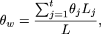where θ_j is the θ value associated with sequence-type j, L_j is the number of bases of type j examined, t is the number of sequence types from Table 2 that were included in the experiment, and . Finally, the “variant-specific θ,” θ_v, considers the evolutionary and positional characteristics of the variant of interest (the potential disease-causing mutation). To calculate θ_v, choose the appropriate θ value from Table 2, using as much information as is known about the variant. If the nucleotide at which the variant occurs is conserved in mice or fugu, multiply θ by the probability of conservation, found in the last two columns of Table 2. With the variant-specific method, L is equal to the number of bases sequenced that are of the same type as the variant of interest. Numerical examples of θ_w and θ_v are given in the Supplemental material.

The true P-value probably lies somewhere between the θ_w and θ_v P-values. The θ_w P-value considers the scope of the entire, but does not account for the positional or evolutionary characteristics of any particular variant. Using θ_w, a variant that causes a nonsynonymous amino acid change has the same P-value as a variant in an intergenic region. In a sense, this P-value is averaged over the entire region examined and probably underestimates the significance of the finding. On the other hand, the θ_v P-value most likely overestimates the significance of the finding. This is because using θ_v considers only the characteristics of the variant of interest and ignores other types of sequence examined for the purpose of identifying the variant.

The methods presented here can be used to guide the selection of an appropriately sized control group for a mutation-detection study. At present, control group size appears to be arbitrary, with 100 chromosomes being a popular choice (Colomb et al. 2003; DiFonzo et al. 2003; Eng et al. 2003; Henneke et al. 2003; Isidro et al. 2003; Kramer et al. 2003; Njalsson et al. 2003; Royer et al. 2003). Examination of the “Mutation in Brief” section of two recent issues of Human Mutation (volume 22, issues 6 and 7) revealed that eight of 11 mutation-detection experiments screened 100 or fewer control chromosomes for a putative disease-causing mutation that was initially found in a patient. The popularity of the 100-chromosome control group may have its roots in the definition of a “polymorphism” as a variant with frequency 1% or higher in the general population. This idea is often attributed to Ford (1965), who asserts that any variant found at frequency 1% or higher in the general population cannot be strictly deleterious. However, the converse of this statement is not true. Occurrence of the variant on <1% of chromosomes does not, per se, indicate that it is likely to be deleterious. In fact, as Table 1 shows, the majority of neutral variants have frequency under 1% in the human population.

For complete resequencing of the average human gene, which may be ∼10 kb in size including exons, intron/exon boundaries, and 5′ and 3′ UTRs, the probability of finding a neutral variant in a patient and not in 100 control chromosomes is about 0.14, indicating that discovery of a novel variant in a patient and not in a relatively small group of controls is, on its own, very weak evidence of involvement with disease. In the absence of information on conservation across species, almost 400 control chromosomes would be required to reduce the P-value to <0.05 for a 10-kb sequence.

The multiple-testing issue is present in the screening of a gene whose product is known to be involved in the development of a disease, in the testing of a candidate gene suspected to be involved in the disease, and in the exploration of the region under a linkage peak. In the investigation of a candidate gene, it would not be unusual to sequence 20 kb in order to identify variants for use in a case-control analysis. Examining 20 kb of sequence increases a nominally significant traditional case-control P-value by almost two orders of magnitude. Resequencing efforts of this scope are currently feasible; 5 kb can be resequenced in ∼100 individuals on 96-well plates in about a week.

Our case-control results are consistent with a traditional case-control analysis when sequence length is taken into account. This consistency allowed the development of a novel, biologically relevant way to adjust for multiple testing in a case-control experiment. P-values obtained using equations 4, 5, or 7 can be approximated by multiplying the traditional case-control P-value by the number of polymorphic sites expected in the region sequenced in the patient group. This method differs from a traditional Bonferroni correction, as the number of sites expected may or may not be equivalent to the number of tests performed. We used equation 6, (1)/(i) (Watterson 1975), to estimate the expected number of polymorphic sites across the region in a sample of N patients (2N chromosomes). We recommend this new simple method for adjusting for multiple testing in a case-control study, as it is easy to apply and yields P-values that are on the order of those obtained via the more complex method.

It should be noted that for the theoretical portion of this work, an equilibrium neutral population of approximately constant effective size is assumed. We have made this simplifying assumption because there are few known analytical results for any other situation. However, since the global human population has expanded in size and humans tend to exhibit an excess of rare alleles relative to an equilibrium population, our tests could be anticonservative. Using simulation, we have shown that, in fact, modeling an expanding population does lead to an excess of rare alleles and to a slightly anticonservative P-value using our method, as shown in Table 3. In part, to compensate for this, throughout this work, we have chosen to use Watterson's (1975) estimator for θ because it tends to be more sensitive to the number of rare sites than other estimators (Tajima 1989). In the most naive approximation imaginable, one might be able to compensate for the observed excess of rare sites in the true human population by an upward adjustment to θ (Slatkin and Hudson 1991). In our data set (Cutler et al. 2001), and in nearly all other human data sets (Ptak and Przeworski 2002), the ratio of Watterson's estimator to Tajima's estimator is seldom larger than a factor of 2, as Tajima's estimator is dominated by high-frequency alleles, with rare SNPs giving little contribution. Therefore, we might believe that the use of equilibrium theory is reasonable, although it is certainly not ideal. This area clearly deserves more careful analysis.

To summarize, here we provide the first sampling theory for assessing the significance of a mutation detection experiment in a rigorous manner. We recommend the following methods.

1. Estimate θ_w, θ_v or use the genome-wide average value of 8.25 × 10^-4.

2. For a simple mutation detection experiment, with either a heterozygous or homozygous outbred patient, estimate a minimum P-value using equation 2 and estimate a maximum P-value using equation 3.

3. If the patient is inbred and f can be estimated, use P₃ and P₃' (online) to estimate minimum and maximum P-values, respectively, or use Supplemental Table 3 to guide selection of an appropriately sized control group.

4. In a case-control study, adjust for multiple testing by multiplying the raw P-value obtained through traditional case-control methods by the number of segregating sites expected in the region resequenced using equation 6.

5. As derived and discussed in the Supplemental material, treat the assertion of disease due to compound heterozygosity with caution, as the probability of identifying a pair of sites heterozygous in a patient and not in controls is extremely high, regardless of the length of sequence examined.

One limitation of our method is its lack of a clear treatment of linkage disequilibrium. For the sake of tractability, we have sometimes assumed both no recombination and free recombination between sites within the same calculation. We have not attempted to realistically model linkage disequilibrium, as this would add extraordinary complexity to the calculations and would almost certainly be inaccurate in any given situation. A second limitation is our lack of consideration of selection. In deriving the expected distribution of allele frequencies, we assumed that new mutations are unrelated to the disease in question and are selectively neutral. Allowing for selection for or against new alleles would distort the expected frequency distribution as a function of the selection parameters.

In spite of these limitations, our method provides a first approximation of the probability of discovering a neutral variant that is over-represented in cases relative to controls. Any P-value calculated using our method should be regarded as one of many lines of evidence in a mutation-detection study. The work presented here is primarily intended to serve as a guideline in determining the appropriate control group size as a function of the length of sequence examined to identify candidate variants and to assist in assessing the significance of a putative mutation.