Single-cell sequencing data reveal widespread recurrence and loss of mutational hits in the life histories of tumors

Jack Kuipers; Katharina Jahn; Benjamin J. Raphael; Niko Beerenwinkel

doi:10.1101/gr.220707.117

Abstract

Intra-tumor heterogeneity poses substantial challenges for cancer treatment. A tumor's composition can be deduced by reconstructing its mutational history. Central to current approaches is the infinite sites assumption that every genomic position can only mutate once over the lifetime of a tumor. The validity of this assumption has never been quantitatively assessed. We developed a rigorous statistical framework to test the infinite sites assumption with single-cell sequencing data. Our framework accounts for the high noise and contamination present in such data. We found strong evidence for the same genomic position being mutationally affected multiple times in individual tumors for 11 of 12 single-cell sequencing data sets from a variety of human cancers. Seven cases involved the loss of earlier mutations, five of which occurred at sites unaffected by large-scale genomic deletions. Four cases exhibited a parallel mutation, potentially indicating convergent evolution at the base pair level. Our results refute the general validity of the infinite sites assumption and indicate that more complex models are needed to adequately quantify intra-tumor heterogeneity for more effective cancer treatment.

The presence of mutational heterogeneity within tumors due to somatic cell evolution is known to be a major cause of treatment failure (Ding et al. 2012; Greaves and Maley 2012). With the emergence of next-generation sequencing techniques, it is possible to systematically analyze individual tumors at a genetic level from admixed cell samples and, more recently, from sequencing the DNA of individual tumor cells (Navin 2014; Van Loo and Voet 2014). These technical advances, together with a prospect of high-precision cancer therapies, have spurred the development of a variety of computational approaches to reconstruct not only the clonal structure but also the entire mutation history of individual tumors (Strino et al. 2013; Hajirasouliha et al. 2014; Jiao et al. 2014; Kim and Simon 2014; Qiao et al. 2014; Deshwar et al. 2015; El-Kebir et al. 2015; Malikic et al. 2015; Niknafs et al. 2015; Popic et al. 2015; Yuan et al. 2015; Jahn et al. 2016; Jiang et al. 2016; Ross and Markowetz 2016; Donmez et al. 2017). A common feature of all these approaches is the infinite sites assumption (ISA) (Kimura 1969) to exclude the possibility of the same genomic site being hit by multiple mutations throughout the lifetime of a tumor. However, the ISA has never been explicitly tested with sequencing data in the context of tumor evolution. Only in the context of copy number alterations has it been recently suggested to allow multiple changes of the same site while still excluding recurrences of the same state (El-Kebir et al. 2016; McPherson et al. 2016).

The ISA is convenient as it substantially restricts the search space of possible mutation histories (Gusfield 1997), but its validity is unproven and difficult to evaluate, as many factors such as mutation rate, cell division rate, copy number changes, and the presence of mutational hotspots influence the probability of multiple mutations hitting the same site. On larger scales, multiple mutations have been observed to affect the same gene at different genomic sites in different spatial areas and phylogenetic branches of tumors (Gerlinger et al. 2012; Kovac et al. 2015; Yates et al. 2015), indicating convergent evolution for these driver genes. Distinct copy number alterations have also been observed to affect the same genes in ovarian cancer (McPherson et al. 2016). This raises the question of whether recurrence even at the scale of individual bases, and corresponding violations of the ISA, can arise during tumor evolution.

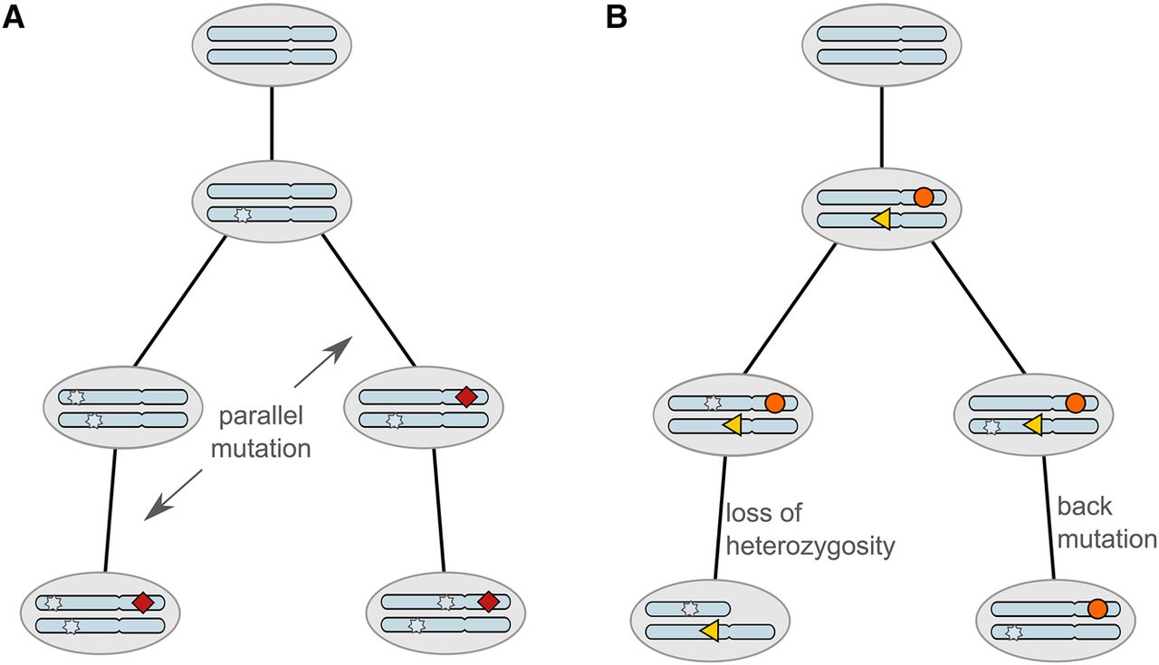
There are two distinct types of recurrences: parallel mutations of the same genomic position undergoing the same substitution independently in different lineages, and back mutations of the same position reverting to its earlier state corresponding to a second hit in the same lineage. Mutations may however also be lost through deletions of the genomic region containing the mutation. Operating on a larger scale than the original point mutation, this does not strictly contradict the assumption of genomic sites only mutating once. However the ISA, by precluding back mutations, implies mutations persist in the phylogeny once they have arisen. Any loss of mutations violates persistence and invalidates the use of the ISA in modeling the phylogeny. Parallel mutations and genuine back mutations directly violate the ISA.

In fact, the idea that every genomic position mutates at most once over the lifetime of a tumor can be disproved by a generalization of the birthday problem (Supplemental Material). This is a classic math puzzle that asks for the probability that two people in a group share the same birthday. Perhaps surprisingly, this probability is already greater than 0.5 with only 23 people. Using the same reasoning and estimates of the cumulative number of stem cell divisions (Tomasetti and Vogelstein 2015) and mutation rates (Lynch 2010), we found that the probability of violating the ISA in any tissue is almost 1 (Supplemental Material).

It is a different question, however, whether the recurrence of mutations is likely to be observed in practice. For bulk studies of admixed samples of cell, violations of the ISA may be obscured since mutational profiles are amalgamated before sequencing. They may therefore be challenging to detect when deconvolving the sample and reconstructing the tumor phylogeny. Single-cell sequencing instead offers the potential to directly observe mutational patterns inconsistent with the ISA. However, from the limited number of tumor cells that are typically sequenced, only a small fraction of mutations may be observed, and only that part of the evolutionary history may be reconstructable. So although it is almost certain that the ISA is violated within the tumor tissue in many cancers, there may still be a low chance to detect a violation among a small set of mutations observed in a small sample of cells (Supplemental Material). The chance will however be increased by any nonuniformity in the underlying mutation rate, which can be affected by a variety of processes, including proximity to breakpoints (Drier et al. 2013), replication timing (Stamatoyannopoulos et al. 2009), and chromatin organization (Schuster-Böckler and Lehner 2012). On the other hand, mutations with a selective advantage leading to tumor growth will be inherited by the corresponding tumor cells making them more likely to be observable. Random passenger mutations present before any expansion will also be similarly amplified across many cells and easier to detect. Selection potentially affects the set of mutations observed in single-cell sequencing data and may affect the chance of recurrent mutations.

Therefore in this paper, we develop a statistical framework based on real tumor data to test the ISA. The method utilizes the power of single-cell sequencing to learn high resolution pictures of tumor evolution and accounts for the noise in such data. We validate the method with simulation studies and then examine a variety of single-cell sequencing data sets, uncovering widespread violations of the ISA in human cancers.

Results

Overview of the method

To identify parallel mutations (Fig. 1) that violate the ISA, or mutational loss that invalidates its use in modeling tumor phylogenies (Supplemental Fig. 1), we built a method (Fig. 2) to test the infinite sites model (ISM), $M_{I}$ , that comprises all histories with a single event for every mutated site, against a model $M_{F}$ that allows multiple mutations at the same site, referred to as the finite sites model (FSM) (Methods). To compare the two alternative models, we compute the Bayes factor (BF) (Kass and Raftery 1995; Moffa et al. 2016) based on single-cell sequencing data, D

B_{FI} = \frac{P (D | M_{F})}{P (D | M_{I})} .

Figure 1.

Somatic mutations occurring during tumor evolution could violate the infinite sites assumption. (A) The mutation indicated by the red diamond occurs in parallel in two different lineages. (B) The mutation depicted by the orange circle is lost in the left branch due to a loss of heterozygosity. The mutation drawn as a yellow triangle is lost in the right branch by reverting to its original state, denoted a back mutation.

Open in new tab Download PowerPointLink to figure

Figure 2.

Testing the infinite sites assumption starts from the single-cell mutation data. The data are examined under both the infinite sites model of all trees with no recurrent mutations as well as under the finite sites model of trees with one recurrence. The two competing models of tumor evolution are compared on how well they explain the single-cell data, with one model selected via the Bayes factor.

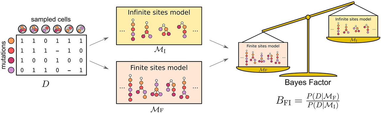
Open in new tab Download PowerPointLink to figure

When the FSM fits the data better than the ISM, the BF is greater than 1, and the larger the value, the stronger the evidence is against the ISA. The BF can be combined with estimates of the prior odds of each model to provide the posterior odds

\frac{P (M_{F} | D)}{P (M_{I} | D)} = B_{FI} \frac{P (M_{F})}{P (M_{I})} .

The computation of the BF requires reconstructing evolutionary histories from mutation profiles of single cells when we also allow a single recurrent mutation (Methods). The recurrent mutation can be either a lost mutation, if the second event occurs in the same cell lineage, or a parallel mutation that occurs in a different lineage (Fig. 1). The reconstruction accounts for the noise in single-cell sequencing data, particularly the high levels of allelic dropout.

Single-cell sequencing data can additionally be contaminated by doublets, the inadvertent sequencing of more than one cell together, with some platforms having rates as high as 40% (Fluidigm 2016). We observed that high doublet contamination rates affect the quality of the reconstructed mutation histories and thereby can confound the model selection process. Therefore we extended both models to account for doublets and to learn their incidence rates from the data (Methods).

In accounting for the noise in singe-cell sequencing data, our approach distinguishes between the random effects of doublets and allelic dropout from the consistent effect on entire lineages of the phylogeny of violations of the ISA. In comparing the model with recurrence to the infinite sites model, the BF quantifies the strength of the consistent effect and hence the improvement of the finite sites model in explaining the data.

Summary of simulation results

Evaluation of our framework on simulated data sets with realistic noise levels and contamination with doublets revealed that our test has a high specificity of 90%–95% using a BF cutoff of 1 (Supplemental Material). The sensitivity increases with the number of sequenced cells. With 2–3 cells per mutation, we find a moderate sensitivity of 50%–60% with the same BF cutoff. Although this means that some recurrent mutations will be overlooked, any signaling of violations of the infinite sites assumption in real data can be trusted.

Overview of single-cell data sets

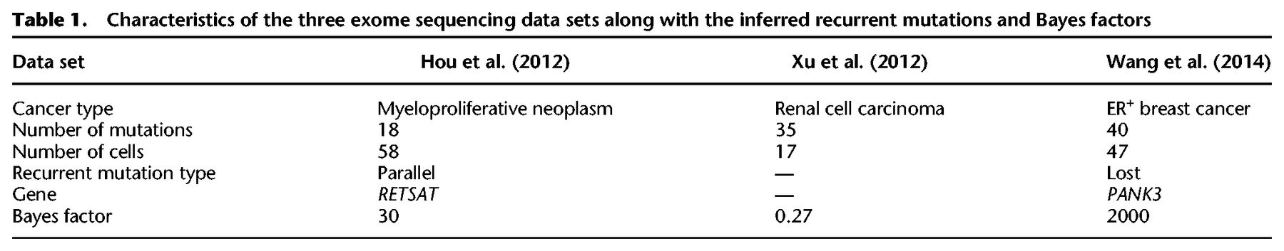
We analyzed 12 published single-cell tumor data sets, three from whole-exome sequencing (Table 1) and nine from targeted sequencing (Tables 2, 3). The details of the inferred parameters and trees are discussed in the Supplemental Material, with the results presented below.

Table 1.

Characteristics of the three exome sequencing data sets along with the inferred recurrent mutations and Bayes factors

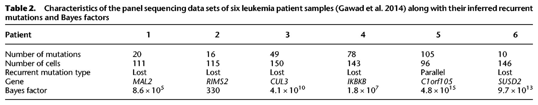
Open in new tab Download PowerPointLink to table

Table 2.

Characteristics of the panel sequencing data sets of six leukemia patient samples (Gawad et al. 2014) along with their inferred recurrent mutations and Bayes factors

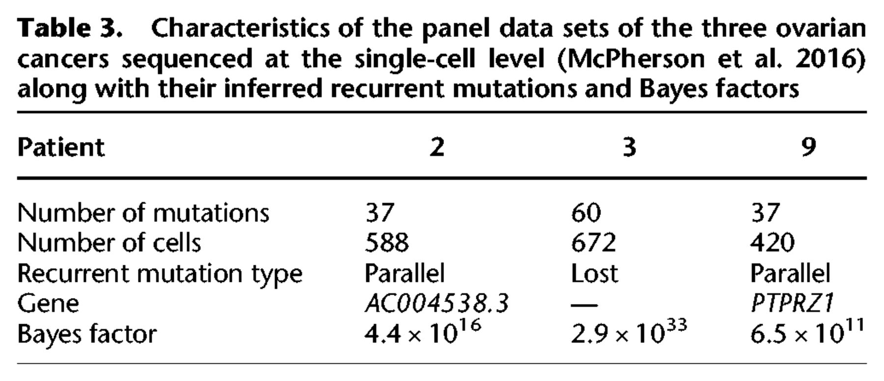
Open in new tab Download PowerPointLink to table

Table 3.

Characteristics of the panel data sets of the three ovarian cancers sequenced at the single-cell level (McPherson et al. 2016) along with their inferred recurrent mutations and Bayes factors

Open in new tab Download PowerPointLink to table

Evidence for recurrent mutations in single-cell exome sequencing data

Looking at a JAK2-negative myeloproliferative neoplasm (essential thrombocythemia) for which the exomes of 58 tumor cells were sequenced, we focused on the 18 mutations classified as cancer-related (Hou et al. 2012) and found evidence for a recurrence of the same point mutation in the RETSAT gene (Supplemental Fig. 13). Both mutations are late events that have happened at the end of two neighboring branches. This recurrence is supported by a BF estimate of 30, constituting reasonable evidence for a violation of the ISA.

Next, we analyzed a clear cell renal cell carcinoma for which exome sequencing data of a total of 17 tumor cells are available (Xu et al. 2012). Performing the model comparison based on the 35 sites informative for mutation tree reconstruction, we obtain a BF below 1. There is therefore no evidence for a violation of the ISA, although any such violation would be hard to detect with the low number of sequenced cells.

In a data set of 47 cells of an estrogen-receptor positive (ER⁺) breast cancer with 40 informative mutation sites (Wang et al. 2014), we found that the tree topology under both models consists of a linear chain of mutations on top of a rather branched structure further down (Supplemental Fig. 15). Under the FSM, a loss of the early PANK3 mutation changes the upper tree structure substantially compared to the tree under the infinite sites model, in which the mutation is forced into a side branch. Computing the BF, we find a value of 2000, providing very strong evidence that the model with loss fits the data much better than the infinite sites model.

For the small number of cells sequenced, and assuming a uniform distribution of mutations with no selection and that all mutations are observed, we obtain the conservative estimate of the probability of the same site among 40 changing twice via point mutations to be rather small at 2.5 × 10⁻⁵ (Supplemental Table 7). We therefore tested loss of heterozygosity (LOH) as an alternative explanation to back mutation: If the only allele carrying the mutation is lost at some point in the tree, sequencing descendant cells will only yield reads from the normal allele thereby mimicking a back mutation (Fig. 1). Based on copy number data from breast cancer samples from The Cancer Genome Atlas (TCGA) Research Network (http://cancergenome.nih.gov/), LOH on the PANK3 gene occurred with a probability of approximately 2 × 10⁻³ and thereby much higher than for the uniform reversion of a point mutation among 40. Copy number estimates are also provided (Wang et al. 2014) for a second set of sequenced cells, although it is difficult to determine whether LOH has occurred in the respective region. The reason for this is because PANK3 is located on Chromosome 5, which was amplified early in the tumor evolution. Of the sequenced cells, most of them seem to still exhibit an amplification of Chromosome 5, but this is less certain for all cells. Some cells may then have lost a copy later, giving a possible explanation of our observation of the mutational loss.

Evidence for recurrent mutations in single-cell panel data

We found strong evidence against the ISA in single-cell sequencing data from the personalized panels of six childhood acute lymphoblastic leukemia (ALL) patients (Gawad et al. 2014). Our test returns extremely high BFs in the range of 10⁵–10¹⁵ (Table 2) for five of the cases and a more modest, but still highly significant, BF estimate of 330 for one patient sample (patient 2). For all samples apart from patient 5, the recurrent mutation is a lost mutation. Looking at the trees (Supplemental Figs. 16–21), we notice that for three patients, the lost mutation is actually the first one that happened in their trees: They affect the MAL2 gene in patient 1, RIMS2 in patient 2, and SUSD2 in patient 6. For patient 4, the lost mutation was in IKBKB, which was also acquired in the tree trunk, whereas the last case, patient 3, lost a mutation in CUL3 that was acquired further down in a branch of the tree. Three of the five lost mutations occur on Chromosome 8.

Because LOH events are the most likely causes of mutational loss, we compared the lost mutations to the 16 LOH events (>10 kb) detected from the bulk data of the six leukemia patients (Gawad et al. 2014). However, the single-cell data showed that the large majority (13 of 16) appeared in all clones and were ancestral (Gawad et al. 2014). None of the five lost mutations we identified appeared in any of the LOH regions of the respective patient, emphasizing that they are unlikely to be the result of large-scale deletions. The data then indicate either smaller scale deletions or genuine back mutations with a reversion of the individual locus.

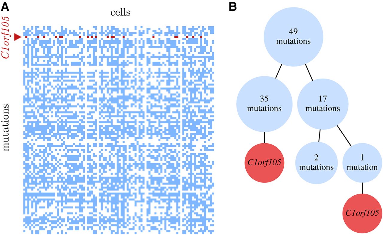
For patient 5, we observed (Fig. 3) a parallel mutation in C1orf105 with a BF of 4.8 × 10¹⁵, so that allowing the mutation to occur twice explains the data much better than enforcing the ISA. Since sequencing bias is an unlikely explanation for the extreme BF, based on analyzing the read counts in the cells (Supplemental Material), our conclusion is that we are observing here a real signal of the same genomic position mutating twice in different subpopulations of a tumor.

Figure 3.

(A) The data matrix of the 105 mutations detected in the 96 single cells of patient 5 of the leukemia data set (Gawad et al. 2014). Unmutated positions are white, mutations are blue, and the recurrent mutation in C1orf105 is red. (B) The inferred mutational history under the finite sites model, when allowing a recurrence of the point mutation in C1orf105. The two occurrences appear at the ends of different lineages in the tree, separated in the two branches by 35 and 18 other mutations. The very large Bayes factor of 4.8 × 10¹⁵ shows that allowing the parallel mutation fits the data much better than enforcing the infinite sites assumption.

Open in new tab Download PowerPointLink to figure

We further analyzed the three single-cell panel sequencing data sets from a cohort of seven ovarian cancer patients (McPherson et al. 2016). For targeted panels of 43 or 84 mutations, between 420 and 672 cells were sequenced, offering a lot of power to detect possible violations of the ISA. The panels included ancestral mutations lost in the tumors, which were excluded for testing the ISA (Supplemental Material). For all three data sets, we indeed find strong evidence against the use of the ISA (Table 3). Patient 3 exhibited a lost mutation on Chromosome 5 outside of the exome in a region detected as suffering from LOH by McPherson et al. (2016). The mutation in the gene PTPRZ1 in patient 9 occurs in parallel, but on the full set of 43 mutations including those with ancestral LOH events, the recurrent mutation fits better as lost during the evolution of the tumor. The mutation is however in a region unaffected by LOH events (McPherson et al. 2016) so that smaller-scale deletions or a back mutation could be an alternative explanation to the parallel mutation observed. Finally, for patient 2, we uncovered an unambiguous parallel mutation affecting the gene AC004538.3.

Signs of secondary parallel mutations

Because lost mutations violate the ISA but may have a simpler biological cause from LOH than a back mutation of the single genomic position reverting, we wished to examine parallel mutations more closely because these act at the level of individual bases. In particular, we restricted our search to consider only the highest scoring parallel mutation for each data set. This may reveal additional violations of the ISA.

For the exome data, the recurrent mutation uncovered from the myeloproliferative neoplasm (Hou et al. 2012) is already parallel, and no other parallel mutation scored highly. No evidence for infinite sites violations was discovered for the kidney cancer (Xu et al. 2012), and for the breast cancer samples (Wang et al. 2014) no parallel mutation scored highly. For the leukemia panel data (Gawad et al. 2014), on the other hand, we find parallel mutations for patients 1–4 with BFs larger than 1 (Supplemental Table 5). Three of them have moderate BFs, but for patient 3, we find a large BF of 2.4 × 10⁶, which indicates multiple violations of the infinite sites hypothesis.

For patient 5, we also found multiple parallel mutations. The top-scoring recurrence was already a parallel mutation (Table 2), but the second highest scoring recurrence is also parallel with a very large BF of 4.1 × 10¹⁰. That mutation occurs on Chromosome 9 at position 139923258 (hg19), which is at the ends of the ABCA2 and C9orf139 genes.

For the ovarian cancer panel data (McPherson et al. 2016), we also find secondary highly scoring parallel recurrences: Chromosome 7 at position 121577182 (hg19) in gene PTPRZ1 with a BF of 4.4 × 10¹³ for patient 2; Chromosome 5 at position 52077065 (hg19) in gene CTD-2288O8.1 with a BF of 5.8 × 10¹⁸ for patient 3; and Chromosome 8 at position 114225881 (hg19) in gene CSMD3 with a BF of 3.2 × 10¹¹ for patient 9.

Discussion

We have developed a statistical framework to test the infinite sites assumption in single-cell sequencing data. Application of our framework to published patient data—one myeloproliferative neoplasm (Hou et al. 2012), one renal cell carcinoma (Xu et al. 2012), one breast tumor (Wang et al. 2014), six leukemia patients (Gawad et al. 2014), and three ovarian cancers (McPherson et al. 2016)—suggests that the assumption is frequently violated. We showed that these findings cannot be explained by the background mutation rate alone, because the prior probability of mutating the same base twice among a selected set of bases is low if mutations are spread uniformly across the genome (Supplemental Table 7).

Most of the observed violations of the infinite sites assumption present as lost mutations, typically as the loss of an early clonal mutation. This may be the result of random losses of passenger mutations, but observing this pattern in many patient samples would also be compatible with selection driven by the microenvironmental or the genetic context. For example, early driver mutations may become obsolete once the tumor is established, or may even hinder the tumor at later stages so their loss becomes positively selected for. Hints of changing selective pressures on particular aberrations have recently been observed for Barrett's esophagus (Martinez et al. 2016). Loss of a copy of CDKN2A seemed to provide a fitness advantage for clones experiencing acid reflux but a disadvantage when the acid is suppressed under treatment. Clones that regain the CDKN2A copy could then potentially experience positive selection. Single-cell sequencing at different time points, or under different treatment pressures, offers a powerful tool for elucidating the underlying tumor evolution and its selective environment, especially when coupled with models like ours, which allow violations of mutational persistence.

A simpler explanation than back mutations for mutational loss is LOH, the loss of a chromosomal segment that comprises a mutated site. In tumors rich in copy number alterations, such an event would have a reasonably high prior probability, because the same site is much easier hit by two or more such large-scale alterations than by two point mutations. In the leukemia data set (Gawad et al. 2014), the lost mutations we identified did not occur in genomic regions affected by large-scale deletions. For half of the leukemia patients, the lost mutation occurs on Chromosome 8, pointing to a particular role in the development of the disease. Although our findings on the incidence of lost mutations are limited to the small number of patient samples available at this point, they may be of importance in the context of treatment strategies that target early trunk mutations in cancer therapy. Our method can be used to generate the trunk mutations more accurately, as evident particularly for the breast cancer sample (Supplemental Fig. 15; Wang et al. 2014).

We also found evidence for parallel mutations in four of the studied cases: the JAK2-negative myeloproliferative neoplasm (Hou et al. 2012), patient 5 of the leukemia data set (Fig. 3; Gawad et al. 2014), and patients 2 and 9 of the ovarian cancer data set (McPherson et al. 2016). Having corrected for the possibility of doublet samples in our model, the event of a mutation hitting the same site twice appears here to be the most plausible explanation; although for patient 9 of the ovarian cancer data set (McPherson et al. 2016), the recurrent mutation could possibly be a loss (Supplemental Material). Conservative estimates of the prior odds of recurrent mutations among a small set of mutations of interest were obtained by spreading mutations uniformly across the genome and assuming that all mutations are observed (Supplemental Table 7). With these low prior estimates, the posterior probability of the infinite site hypothesis is still larger for the exome data of the myeloproliferative neoplasm (Hou et al. 2012). For patient 2 of the ovarian cancer data set (McPherson et al. 2016) and for patient 5 of the leukemia panel data (Gawad et al. 2014), the BF is large enough that the posterior odds are certainly in favor of the infinite sites hypothesis being violated. These data are then the “smoking gun,” showing that the possibility of infinite sites violations needs to be seriously considered and treated for single-cell data. Again, larger sample sizes will be needed to better assess the practical implications of these findings, but modeling single-cell data while allowing violations of the infinite sites hypothesis provides the statistical framework for exactly that.

The possibility of violations of the infinite sites assumption necessitates substantial adaptations in present-day models for reconstructing mutation histories of tumors. For example, in models designed for bulk sequencing data, a core assumption to deconvolve admixed mutation profiles is that the cellular frequency of a point mutation distributes over a single clade in the tumor phylogeny, a restriction that is contrary to the recurrence of a mutation in different parts of the tree. When looking at models based on single-cell data such as SCITE (Jahn et al. 2016), the changes necessary to accommodate finite sites seem less profound, as indicated by the extension introduced in this paper to allow a single recurrent mutation. We also used this method to search for multiple recurrences by restricting the recurrence to parallel mutations in data in which higher scoring lost mutations had been observed. This uncovered evidence of multiple violations of the ISA, but a strict statistical test would need to account for the higher scoring recurrences as well. However, the generalization toward the recurrence of an unknown number of mutations in unknown multiplicities entails a vast extension of the underlying search space.

For single-cell data, we additionally have the issue of high doublet rates, which can severely affect reconstruction quality when not being explicitly modeled. Although the accidental sequencing of more than one cell could be relatively easily prevented by rigorously checking samples prior to sequencing, it is likely to take some time before this issue is solved reasonably well for all technology platforms, including high-throughput assays. Meanwhile, it is essential to integrate doublets in models for reconstructing mutation histories from single-cell data. Especially for testing the ISA, modeling doublets is necessary, since even a small number of doublets can interfere with the test. As we have shown in this work, modeling doublets is straightforward for a mutation-centric approach like SCITE (Jahn et al. 2016). For sample-centric approaches such as BitPhylogeny (Yuan et al. 2015) and OncoNEM (Ross and Markowetz 2016), the integration of doublets may be a bit more involved, as the topology underlying the evolutionary history is no longer tree-like in the presence of admixed samples.

Along with accounting for doublet contamination, our modeling deals with the typical noise in single-cell sequencing data, especially high false negative rates from allelic dropout and missing data from a lack of coverage. In testing the ISA, our method disentangles consistent effects of violations of the ISA from random sequencing noise. Particularly for targeted sequencing, however, certain primers may be less effective than others. This may lead to higher rates of missing data and introduce correlations in the mutational noise profiles across cells. Tackling such correlations with a more granular approach could be an interesting extension of our approach. The error model we used, however, can also be viewed as allowing full granularity of each mutation in each cell having its own error profile, drawn independently from the same underlying distribution.

We focused in this work on testing the infinite sites assumption for point mutations in tumor evolution. This extends more generally to any cell lineages and their phylogeny, where we know that violations become increasingly likely for larger sets of cells and mutations. Looking at larger-scale lesions in cancer, such as copy number alterations, the importance of allowing recurrent mutations becomes even more pronounced. These alterations typically affect larger segments, which make it much more likely that the same site is affected multiple times. To model this type of lesion, either alone or together with SNVs to integrate LOH, dropping the infinite sites assumption becomes even more crucial. Outside of tumor evolution, substitution models allowing recurrent mutations have been well developed and efficiently implemented (Ronquist et al. 2012; Bouckaert et al. 2014; Stamatakis 2014) but do not directly account for the mixing of clones in bulk samples or the noise inherent in single-cell sequencing. For tumor sequencing data, recent work using the less restrictive infinite alleles assumption (El-Kebir et al. 2016), Dollo parsimony with loss (McPherson et al. 2016), or penalizing violations (Marass et al. 2016) are promising first steps. However, additional work on accurate models of tumor evolution and their inference from sequencing data is essential.

Methods

Tree models

The genealogy of somatic cells can be represented as a cell lineage tree, a rooted labeled binary tree, where the leaves represent the cells and the tree structure reflects the cell division history. Tree edges are labeled with mutation events, and all cells below a mutation can be expected to exhibit this mutation, e.g., the left-most tree in Figure 4A.

Figure 4.

(A) Cell lineage trees of seven cells. (Left) No recurrent mutations; (middle) parallel mutation, a mutation occurs twice in separate lineages, denoted as M₃ and $M_{3}^{'}$ , cells below both occurrences exhibit this mutation; (right) lost mutation, a second occurrence of a mutation in the same lineage brings the genomic site back to the original state, i.e., cells located below $M_{1}^{'}$ do not exhibit this mutation. (B) Mutation trees with attached cell samples. Each tree corresponds to the cell lineage tree in the same column. (C) Mutation matrices with binary states, each corresponds to the mutation tree in the same column. Entry (i,j) contains the expected state of mutation M_i in cell s_j, 0 for absence and 1 for presence in the cell. The red zeros in the matrix on the right are due to the placement of cells s₆ and s₇ below $M_{1}^{'}$ , the second occurrence of mutation M₁, which brings the genomic site back to the original state.

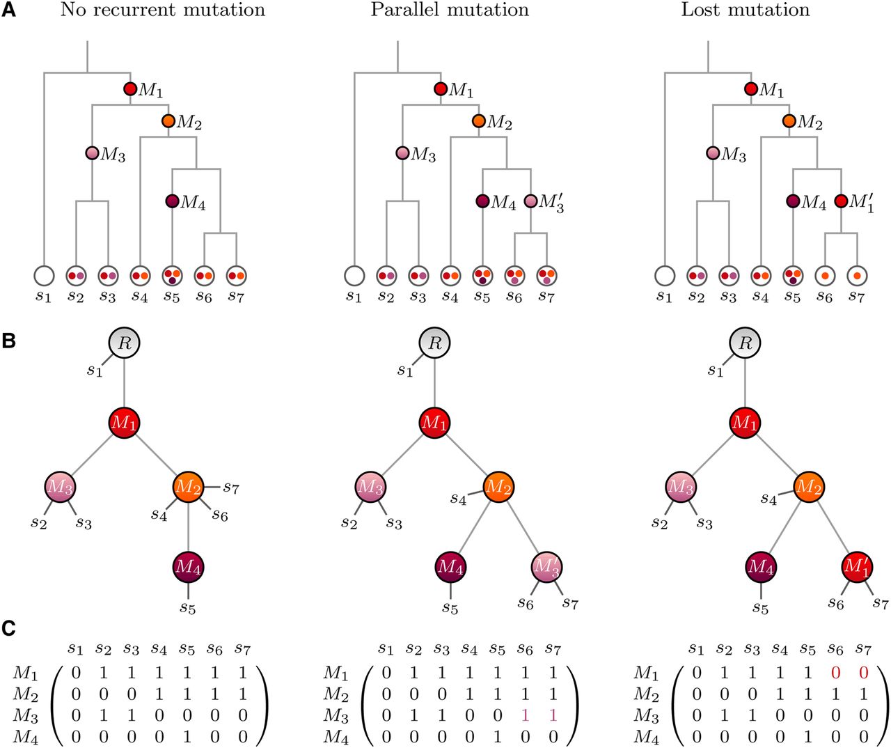
Open in new tab Download PowerPointLink to figure

Models for somatic cell evolution typically make the infinite sites assumption that restricts any genomic site to host no more than one mutation event. Dropping this assumption means allowing not just one but multiple occurrences of the mutations in a cell lineage tree. For simplicity, we allow here just a single mutation to occur twice. If the two copies of the same mutation happen in different branches, we refer to them as parallel mutations. A mutation that occurs twice in the same lineage represents a lost mutation. We interpret this as the second mutation undoing the first mutation such that samples that have two copies of a mutation in their history would not exhibit the mutation, e.g., Figure 4A.

In SCITE (Jahn et al. 2016), we utilized mutation trees as an alternative representation of mutation histories. The mutations form the tree nodes that are connected based on their partial temporal order (Fig. 4B). A root is added to define the direction of the tree. Cell samples may attach to any of the nodes, and we expect them to contain all mutations on the path from the root to their attachment point. As with cell lineage trees, we can have parallel and lost mutations. The complete mutation history is defined by a pair $(T, σ)$ , where T is the mutation tree and $σ$ is the attachment array in which entry j encodes the node at which sample cell s_j attaches to the mutation tree. For the trees in Figure 4, we have the attachment vectors

(1)

\begin{aligned} σ = (R, M_{3}, M_{3}, M_{2}, M_{4}, M_{2}, M_{2}), \\ σ = (R, M_{3}, M_{3}, M_{2}, M_{4}, M_{3}^{'}, M_{3}^{'}), \\ σ = (R, M_{3}, M_{3}, M_{2}, M_{4}, M_{1}^{'}, M_{1}^{'}) . \end{aligned}

The mutation states of the cell samples can also be represented as a mutation matrix E. Here, entry (i, j) encodes the presence of a mutation M_i in a cell s_j with a 1 and its absence with a 0 (Fig. 4C). In practice, it is not necessary to construct the complete mutation matrix, as its entries can be obtained from T and $σ_{j}$ , the jth entry of the attachment vector. Let ${anc}_{T} (σ_{j})$ be the set of mutations that are ancestors of $σ_{j}$ in T including σ_j itself, then we have

(2)

E_{i j} = {\begin{array}{ll} 1 if M_{i} \in an c_{T} (σ_{j}) \\ 0 otherwise \end{array}

if M_i is a unique mutation. For M_i and M_i^′ being the two instances of a recurrent mutation, we have

(3)

E_{i j} = {\begin{array}{ll} 1 if M_{i} \in an c_{T} (σ_{j}) and M_{i}^{'} \notin an c_{T} (σ_{j}) \\ 1 if M_{i} \notin an c_{T} (σ_{j}) and M_{i}^{'} \in an c_{T} (σ_{j}) \\ 0 otherwise \end{array}

to encode the state after the mutation loss as a 0 in the mutation matrix.

Error model

In practice, we observe a noisy version D of the expected mutation matrix E. If the true mutation value is 0, we may observe a 1 with a probability of α (false positive); if the true value is 1, we may observe a 0 with probability β (false negative)

(4)

\begin{aligned} P (D_{i j} = 0 | E_{i j} = 0) = (1 - α), P (D_{i j} = 1 | E_{i j} = 0) = α, \\ P (D_{i j} = 0 | E_{i j} = 1) = β, P (D_{i j} = 1 | E_{i j} = 1) = (1 - β) . \end{aligned}

Missing data do not contribute to the likelihood

(5)

\begin{aligned} P (D_{i j} = NA | E_{i j} = 0) = 1, \\ P (D_{i j} = NA | E_{i j} = 1) = 1. \end{aligned}

Assuming the observational errors are independent of each other, the likelihood of the data given a mutation tree T and knowledge of the attachment of the samples σ is

(6)

P (D | T, σ) = \prod_{i = 1}^{n} \prod_{j = 1}^{m} P (D_{i j} | E_{i j}),

where E is the expected mutation matrix for T and σ. To obtain the marginal tree likelihood independent of attachments, we sum over all attachment vectors σ

(7)

P (D | T) = \sum_{σ} P (D | T, σ) P (σ | T) .

With m cells and n mutations, this can be computed efficiently in time O(mn) (Jahn et al. 2016). Using a uniform prior for the sample attachment, P(σ|T) becomes just a normalization constant that can be taken out of the sum. In the following, we refer to the unnormalized marginal likelihood as the tree score

(8)

s (T) = \sum_{σ} P (D | T, σ) .

Modeling doublets

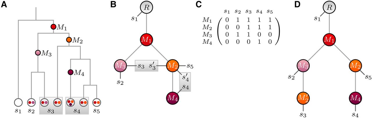
In single-cell sequencing, it can happen that accidentally two (or more) cells are processed together, which generates an admixed mutation profile of these cells (Fig. 5). For our binary mutation states, we assume that a mutation is called whenever it is present in at least one of the cells.

Figure 5.

Tree reconstruction in the presence of doublet samples. (A) Cell lineage tree with doublets (gray boxes). (B) Mutation tree with true sample attachment. Doublet samples (s₃, $s_{3}^{'}$ ) and (s₄, $s_{4}^{'}$ ) each attach to two different nodes. (C) Mutation matrix with combined mutation states for the doublet samples. Mutations are counted as present in a doublet sample if present in at least one of the cells. (D) A tree with a recurrence of mutation M₂ and no doublets is an alternative explanation for the mutation matrix in C.

Open in new tab Download PowerPointLink to figure

The two cells of a doublet sample s_j can attach to different nodes of the mutation tree. Hence we change the attachment vector such that each entry j consists of a pair $(σ_{j}, σ_{j}^{'})$ to indicate the two attachment points. The expected mutation vector is then defined as

(9)

E_{i j} = {\begin{cases} 1 & if M_{i} \in {anc}_{T} (σ_{j}) and M_{i}^{'} \notin {anc}_{T} (σ_{j}) \\ 1 & if M_{i} \notin {anc}_{T} (σ_{j}) and M_{i}^{'} \in {anc}_{T} (σ_{j}) \\ 1 & if M_{i} \in {anc}_{T} (σ_{j}^{'}) and M_{i}^{'} \notin {anc}_{T} (σ_{j}^{'}) \\ 1 & if M_{i} \notin {anc}_{T} (σ_{j}^{'}) and M_{i}^{'} \in {anc}_{T} (σ_{j}^{'}) \\ 0 & otherwise . \end{cases}

To accommodate for doublets in our model, we allow each sample to be a doublet with probability δ and a single cell with probability (1 − δ). To obtain the likelihoods P′(D|T) under this model, we first consider each sample separately. Let D_j be the observed mutation profile of sample s_j, then we denote as

(10)

P_{1} (D_{j} | T) = \sum_{σ_{j} = 1}^{n^{'} + 1} \prod_{i = 1}^{n} P (D_{i j} | T, σ_{j}) P (σ_{j} | T)

the likelihood for sample s_j under the assumption that the sample is a single cell. The use of n′ + 1, instead of n + 1 in the sum, accounts for the changing tree size when recurrences are allowed. For n mutations with a single recurrence, we have n′ = n + 1 tree nodes apart from the root, while n′ = n in case of n unique mutations. Similarly we obtain

(11)

P_{2} (D_{j} | T) = \sum_{σ_{j} = 1}^{n^{'} + 1} \sum_{σ_{j}^{'} = 1}^{n^{'} + 1} \prod_{i = 1}^{n} P (D_{i j} | T, σ_{j}, σ_{j}^{'}) P (σ_{j} | T) P (σ_{j}^{'} | T)

for the case that s_j consists of two cells. To combine the two likelihoods, we weight them by the respective single-cell and doublet probability

(12)

P^{'} (D_{j} | T) = (1 - δ) P_{1} (D_{j} | T) + δ P_{2} (D_{j} | T) .

Then assuming that the sample attachments are independent of each other, the complete likelihood is the product over all samples

(13)

P^{'} (D | T) = \prod_{j = 1}^{m} [(1 - δ) P_{1} (D_{j} | T) + δ P_{2} (D_{j} | T)] .

Because we have to account for all pairings of cell attachments, the time complexity of calculating the likelihood is O(mn²). To obtain a tree score analogous to Equation 8, which is more useful for combinatorial considerations later, we divide the tree likelihood by the prior probability for a single attachment, a factor shared by all terms of the sum

(14)

s (T) = P^{'} (D | T) (n^{'} + 1)^{m} .

Model selection

To test the infinite sites hypothesis, we compare the evidence our observed data D provide in favor of model $M_{I}$ , consisting of trees with unique mutations, and a model that allows for recurrent mutations. For simplicity, we focus here on the model $M_{F}$ with exactly one repeated mutation. Finding strong evidence to favor $M_{F}$ over $M_{I}$ would be sufficient to reject the infinite sites hypothesis. We use Bayes factors for the model selection,

(15)

B_{FI} = \frac{P (D | M_{F})}{P (D | M_{I})} .

A value of B_FI > 1 means that the data are better explained by the finite sites model than by the infinite sites model. The larger the number, the stronger the evidence. To obtain the likelihood under $M_{I}$ , we sum over all mutation trees with a single node for each mutated site observed in D which gives us

(16)

\begin{aligned} P (D | M_{I}) & = \sum_{T \in M_{I}} P (D, T | M_{I}) \\ = \sum_{T \in M_{I}} P (D | T, M_{I}) P (T | M_{I}) \\ = \sum_{T \in M_{I}} P (D | T) P (T | M_{I}) . \end{aligned}

The dependency on $M_{I}$ in P(D|T) can be dropped, as the data are no longer influenced by the model once the tree is fixed. To obtain the tree likelihood, we sum over all attachment vectors, such that

(17)

\begin{array}{l} P (D | M_{I}) & = \sum_{T \in M_{I}} \underset{s (T)}{\underset{⏟}{\sum_{σ} P (D | T, σ)}} P (σ | T) P (T | M_{I}) \end{array} .

The unnormalized marginal tree likelihood is the tree score s(T) as defined in Equation 8. Lastly using a uniform distribution for the prior on trees and sample attachments under a given model, we obtain

(18)

P (D | M_{I}) = \frac{1}{K_{I}} \sum_{T \in M_{I}} s (T),

where K_I is the number of pairs

(T, σ)

belonging to

M_{I}

(19)

K_{I} = (n + 1)^{n + m - 1} .

The finite sites model is the union of models $M_{1}, \dots, M_{n}$ , where each $M_{i}$ comprises all trees in which only mutation i has a second occurrence. We then have

(20)

\begin{matrix} P (D | M_{i}) & = \frac{1}{K_{i}} \sum_{T \in M_{i}} s (T) \end{matrix},

where K_i is the number of pairs

(T, σ)

belonging to

M_{i}

However, for the model comparison, we are only interested in trees that do not just re-create trees from the infinite sites model in the sense that the recurrent mutation does not give rise to any additional mutation profiles compared to a tree without the recurrence. For example, if the recurrent mutation is the direct child or parent of the original copy, or if it shares a parent, then the recurrence can be removed. Excluding such trees from consideration and our model space leads to

(21)

K_{i} = \frac{1}{2} (n - 1) (n + 2)^{n - 1 + m},

as derived in the Supplemental Material.

Another simple example is the case in which the recurrent mutation has no descendant mutations and no samples attached to it. Then we recover a tree with no recurrent mutation, and we should also exclude such cases. This possibility however depends on where the samples attach, rather than just on the tree, so it cannot be excluded from the model space without interfering with the marginalization over $σ$ . Instead we include this possibility in our model class, along with further cases discussed in the Supplemental Material, but correct for their effect by deriving an upper bound for the number of trees and attachment pairs in $M_{F}$ that truly make use of the recurrent mutation and use

(22)

{\tilde{K}}_{F} = n [K_{i} - (n - 1) K_{I}] .

Likewise, we obtain lower bounds for the model likelihood and the Bayes factor

(23)

P (D | M_{F}) \geq \frac{1}{{\tilde{K}}_{F}} \sum_{i} [\sum_{T \in M_{i}} s (T) - n e \sum_{T \in M_{I}} s (T)]

and

(24)

B_{FI} \geq \frac{K_{I}}{{\tilde{K}}_{F}} [\frac{\sum_{i} \sum_{T \in M_{i}} s (T)}{\sum_{T \in M_{I}} s (T)} - n^{2} e] .

The derivation of the bounds is detailed in the Supplemental Material.

When calculating the tree scores, we take fixed values for the error rates, either those provided with the data or learned under the infinite sites model. For the double rate δ, for each tree we find the value that maximizes the score with numerical optimization equivalent to the EM algorithm. We also calculate as $\hat{δ}$ the fraction of samples that are doublets involving mutations from two lineages, since doublets from a single lineage could be modeled as singlets instead.

Approximation

Typically there will be one recurrent mutation that increases the likelihood of the finite sites model much more strongly than the others

(25)

i^{*} = \arg max_{i} \sum_{T \in M_{i}} s (T),

so that in the sum over i in Equation 24, the terms for the other

M_{i}

can essentially each be replaced by the sum over the copies of trees inside

M_{I}

and

(26)

B_{FI} \geq \frac{K_{I}}{{\tilde{K}}_{F}} [\frac{\sum_{T \in M_{i^{*}}} s (T)}{\sum_{T \in M_{I}} s (T)} - n e] .

Estimation via MCMC

In general, the sum over all tree scores cannot be computed for the two models because both comprise a vast number of trees, which grows super-exponentially in the number of mutations. Instead we estimate this value for each model using the MCMC scheme developed in SCITE (Jahn et al. 2016) to search the space of rooted mutation trees.

Given the current tree T, we propose a tree T′ from the same model according to one of the three move types with some proposal probability q(T′|T) and accept the move with probability

(27)

ρ = min {1, \frac{q (T | T^{'}) s (T^{'})}{q (T^{'} | T) s (T)}},

so that we obtain (after some burn in time) a sampler that provides trees proportionally to s(T). Running the sampler for enough steps, we will not only find a tree with the best score in a model

M

(28)

T^{*} = arg max_{T \in M} s (T),

but also the total number of trees with the optimal score,

(29)

c (T^{*}) = # {T \in M | s (T) = s (T^{*})} .

In general, the optimal tree will be unique because of the marginalization over the attachment of samples (or we have two equivalent copies with labels swapped in $M_{F}$ ). If two or more mutations appear in exactly the same set of sampled cells (up to missing data), then the number of trees will grow, but equally for both model classes, so the factors of c will cancel anyway. For completeness, however, we treat the arbitrary case here.

For our estimation of the sum score, we now make use of the fact that in a sequence of trees sampled after burn-in, the fraction of optimal trees approximates the ratio between the sum score of all optimal trees and the sum score over the whole tree space:

(30)

\frac{Number of optimal trees sampled}{Number of trees sampled} \approx \frac{c (T^{*}) s (T^{*})}{\sum_{T \in M} s (T)} .

For this approximation to work, we need to know how long the MCMC needs to run until it has certainly converged. Then the chain of each run is equally likely to discover each of the maximally scoring trees. With the number of currently discovered maximal trees and the probability of discovering each of them in a run (or per state in the chain and the correlation between states), we can estimate and bound the probability that we are still missing any maximally scoring trees (or even better scoring ones). We can then simply run enough chains to reduce this to very low values.

For the left part of Equation 30, we simply need to know how often we hit a maximal tree in a typical chain. For this, we run the chain several times and record, after a burn in period, the time the chain spends at the maximal score.

Simply running this procedure once for $M = M_{I}$ and once for $M = M_{i^{*}}$ then allows us to find an approximation for the ratio in Equation 26. Running many chains gives confidence intervals on the ratios and hence on the final BFs.

Approximation via s(T)

For some data, the posterior may be very flat, which prohibits sampling of the set of maximum scoring trees in reasonable time. For such cases, we make the approximation that the ratio of sampling the optimal trees in each model class is the same for both model classes so that

(31)

s (T^{*}) \propto \sum_{T \in M} s (T)

with the same proportionality constant for both model classes. Then we can effectively replace the sum over all trees in the BFs by s(T*), the score of a single maximum scoring tree

(32)

{\tilde{B}}_{FI} ≳ \frac{K_{I}}{{\tilde{K}}_{F}} [\frac{s (T^{*} \in M_{i^{*}})}{s (T^{*} \in M_{I})} - n e] .

Finding the maximal score can also be made more efficient by monotonically changing the score landscape (for example, raising the score to some power γ), which can be adapted to speed up the MCMC search.

Acknowledgments

We thank Giusi Moffa for very useful discussions about the Bayes Factor comparison (Moffa et al. 2016); Mykola Lebid for running spatial simulations of tumor evolution (Waclaw et al. 2015); and Jochen Singer for bioinformatics support with the leukemia data (Gawad et al. 2014). J.K. was supported by the European Research Council Synergy Grant 609883 (http://erc.europa.eu/). K.J. was supported by SystemsX.ch RTD Grant 2013/150 (http://www.systemsx.ch/).

Author contributions: J.K. and K.J. developed and implemented the method. All authors conceived and designed the study. All authors drafted the manuscript and approved the final version.

Notes

[1] Supplementary material [Supplemental material is available for this article.]

[2] Article published online before print. Article, supplemental material, and publication date are at http://www.genome.org/cgi/doi/10.1101/gr.220707.117.

References

↵
Bouckaert R, Heled J, Kühnert D, Vaughan T, Wu C-H, Xie D, Suchard MA, Rambaut A, Drummond AJ. 2014. BEAST 2: a software platform for Bayesian evolutionary analysis. PLoS Comput Biol 10: e1003537.
Google Scholar CrossRef PubMed
↵
Deshwar AG, Vembu S, Yung CK, Jang GH, Stein L, Morris Q. 2015. PhyloWGS: reconstructing subclonal composition and evolution from whole-genome sequencing of tumors. Genome Biol 16: 35.
Google Scholar CrossRef PubMed
↵
Ding L, Ley TJ, Larson DE, Miller CA, Koboldt DC, Welch JS, Ritchey JK, Young MA, Lamprecht T, McLellan MD, 2012. Clonal evolution in relapsed acute myeloid leukaemia revealed by whole-genome sequencing. Nature 481: 506–510.
Google Scholar CrossRef PubMed Web of Science
↵
Donmez N, Malikic S, Wyatt AW, Gleave ME, Collins CC, Sahinalp SC. 2017. Clonality inference from single tumor samples using low-coverage sequence data. J Comput Biol 24: 515–523.
Google Scholar
↵
Drier Y, Lawrence MS, Carter SL, Stewart C, Gabriel SB, Lander ES, Meyerson M, Beroukhim R, Getz G. 2013. Somatic rearrangements across cancer reveal classes of samples with distinct patterns of DNA breakage and rearrangement-induced hypermutability. Genome Res 23: 228–235.
Google Scholar CrossRef Abstract/Full Text PubMed Web of Science
↵
El-Kebir M, Oesper L, Acheson-Field H, Raphael BJ. 2015. Reconstruction of clonal trees and tumor composition from multi-sample sequencing data. Bioinformatics 31: i62–i70.
Google Scholar CrossRef PubMed
↵
El-Kebir M, Satas G, Oesper L, Raphael BJ. 2016. Inferring the mutational history of a tumor using multi-state perfect phylogeny mixtures. Cell Syst 3: 43–53.
Google Scholar
↵
Fluidigm. 2016. Doublet rate and detection on the C1 IFCs. White Paper PN 101–2711 A1.
Google Scholar
↵
Gawad C, Koh W, Quake SR. 2014. Dissecting the clonal origins of childhood acute lymphoblastic leukemia by single-cell genomics. Proc Natl Acad Sci 111: 17947–17952.
Google Scholar CrossRef PubMed
↵
Gerlinger M, Rowan AJ, Horswell S, Larkin J, Endesfelder D, Gronroos E, Martinez P, Matthews N, Stewart A, Tarpey P, 2012. Intratumor heterogeneity and branched evolution revealed by multiregion sequencing. N Engl J Med 366: 883–892.
Google Scholar CrossRef PubMed Web of Science
↵
Greaves M, Maley CC. 2012. Clonal evolution in cancer. Nature 481: 306–313.
Google Scholar CrossRef PubMed Web of Science
↵
Gusfield D. 1997. Algorithms on strings, trees and sequences: computer science and computational biology. Cambridge University Press, Cambridge, UK.
Google Scholar
↵
Hajirasouliha I, Mahmoody A, Raphael BJ. 2014. A combinatorial approach for analyzing intra-tumor heterogeneity from high-throughput sequencing data. Bioinformatics 30: i78–i86.
Google Scholar CrossRef PubMed
↵
Hou Y, Song L, Zhu P, Zhang B, Tao Y, Xu X, Li F, Wu K, Liang J, Shao D, 2012. Single-cell exome sequencing and monoclonal evolution of a JAK2-negative myeloproliferative neoplasm. Cell 148: 873–885.
Google Scholar CrossRef PubMed Web of Science
↵
Jahn K, Kuipers J, Beerenwinkel N. 2016. Tree inference for single-cell data. Genome Biol 17: 86.
Google Scholar
↵
Jiang Y, Qiu Y, Minn AJ, Zhang NR. 2016. Assessing intratumor heterogeneity and tracking longitudinal and spatial clonal evolutionary history by next-generation sequencing. Proc Natl Acad Sci 113: E5528–E5537.
Google Scholar CrossRef PubMed
↵
Jiao W, Vembu S, Deshwar AG, Stein L, Morris Q. 2014. Inferring clonal evolution of tumors from single nucleotide somatic mutations. BMC Bioinformatics 15: 35.
Google Scholar CrossRef PubMed
↵
Kass RE, Raftery AE. 1995. Bayes factors. J Am Stat Assoc 90: 773–795.
Google Scholar CrossRef PubMed Web of Science
↵
Kim KI, Simon R. 2014. Using single cell sequencing data to model the evolutionary history of a tumor. BMC Bioinformatics 15: 27.
Google Scholar CrossRef PubMed
↵
Kimura M. 1969. The number of heterozygous nucleotide sites maintained in a finite population due to steady flux of mutations. Genetics 61: 893.
Google Scholar PubMed Web of Science
↵
Kovac M, Navas C, Horswell S, Salm M, Bardella C, Rowan A, Stares M, Castro-Giner F, Fisher R, De Bruin EC, 2015. Recurrent chromosomal gains and heterogeneous driver mutations characterise papillary renal cancer evolution. Nat Commun 6: 6336.
Google Scholar CrossRef PubMed
↵
Lynch M. 2010. Rate, molecular spectrum, and consequences of human mutation. Proc Natl Acad Sci 107: 961–968.
Google Scholar CrossRef PubMed
↵
Malikic S, McPherson AW, Donmez N, Sahinalp CS. 2015. Clonality inference in multiple tumor samples using phylogeny. Bioinformatics 31: 1349–1356.
Google Scholar CrossRef PubMed
↵
Marass F, Mouliere F, Yuan K, Rosenfeld N, Markowetz F. 2016. A phylogenetic latent feature model for clonal deconvolution. Ann Appl Stat 10: 2377–2404.
Google Scholar
↵
Martinez P, Timmer MR, Lau CT, Calpe S, del Carmen Sancho-Serra M, Straub D, Baker AM, Meijer SL, Ten Kate FJ, Mallant-Hent RC, 2016. Dynamic clonal equilibrium and predetermined cancer risk in Barrett's oesophagus. Nat Commun 7: 12158.
Google Scholar
↵
McPherson A, Roth A, Laks E, Masud T, Bashashati A, Zhang AW, Ha G, Biele J, Yap D, Wan A, 2016. Divergent modes of clonal spread and intraperitoneal mixing in high-grade serous ovarian cancer. Nat Genet 48: 758–767.
Google Scholar CrossRef PubMed
↵
Moffa G, Erdmann G, Voloshanenko O, Hundsrucker C, Sadeh MJ, Boutros M, Spang R. 2016. Refining pathways: a model comparison approach. PLoS One 11: e0155999.
Google Scholar
↵
Navin NE. 2014. Cancer genomics: one cell at a time. Genome Biol 15: 452.
Google Scholar CrossRef PubMed
↵
Niknafs N, Beleva-Guthrie V, Naiman DQ, Karchin R. 2015. SubClonal hierarchy inference from somatic mutations: automatic reconstruction of cancer evolutionary trees from multi-region next generation sequencing. PLoS Comput Biol 11: e1004416.
Google Scholar CrossRef PubMed
↵
Popic V, Salari R, Hajirasouliha I, Kashef-Haghighi D, West RB, Batzoglou S. 2015. Fast and scalable inference of multi-sample cancer lineages. Genome Biol 16: 91.
Google Scholar CrossRef PubMed
↵
Qiao Y, Quinlan AR, Jazaeri AA, Verhaak RG, Wheeler DA, Marth GT. 2014. SubcloneSeeker: a computational framework for reconstructing tumor clone structure for cancer variant interpretation and prioritization. Genome Biol 15: 443.
Google Scholar CrossRef PubMed
↵
Ronquist F, Teslenko M, Van Der Mark P, Ayres DL, Darling A, Höhna S, Larget B, Liu L, Suchard MA, Huelsenbeck JP, 2012. MrBayes 3.2: efficient Bayesian phylogenetic inference and model choice across a large model space. Syst Biol 61: 539–542.
Google Scholar CrossRef PubMed
↵
Ross E, Markowetz F. 2016. OncoNEM: inferring tumour evolution from single-cell sequencing data. Genome Biol 17: 69.
Google Scholar
↵
Schuster-Böckler B, Lehner B. 2012. Chromatin organization is a major influence on regional mutation rates in human cancer cells. Nature 488: 504–507.
Google Scholar CrossRef PubMed Web of Science
↵
Stamatakis A. 2014. RAxML version 8: a tool for phylogenetic analysis and post-analysis of large phylogenies. Bioinformatics 30: 1312–1313.
Google Scholar CrossRef PubMed Web of Science
↵
Stamatoyannopoulos JA, Adzhubei I, Thurman RE, Kryukov GV, Mirkin SM, Sunyaev SR. 2009. Human mutation rate associated with DNA replication timing. Nat Genet 41: 393–395.
Google Scholar CrossRef PubMed Web of Science
↵
Strino F, Parisi F, Micsinai M, Kluger Y. 2013. TrAp: a tree approach for fingerprinting subclonal tumor composition. Nucleic Acids Res 41: e165.
Google Scholar CrossRef PubMed
↵
Tomasetti C, Vogelstein B. 2015. Variation in cancer risk among tissues can be explained by the number of stem cell divisions. Science 347: 78–81.
Google Scholar CrossRef PubMed Web of Science
↵
Van Loo P, Voet T. 2014. Single cell analysis of cancer genomes. Curr Opin Genet Dev 24: 82–91.
Google Scholar CrossRef PubMed
↵
Waclaw B, Bozic I, Pittman ME, Hruban RH, Vogelstein B, Nowak MA. 2015. A spatial model predicts that dispersal and cell turnover limit intratumour heterogeneity. Nature 525: 261–264.
Google Scholar CrossRef PubMed
↵
Wang Y, Waters J, Leung ML, Unruh A, Roh W, Shi X, Chen K, Scheet P, Vattathil S, Liang H, 2014. Clonal evolution in breast cancer revealed by single nucleus genome sequencing. Nature 512: 155–160.
Google Scholar CrossRef PubMed Web of Science
↵
Xu X, Hou Y, Yin X, Bao L, Tang A, Song L, Li F, Tsang S, Wu K, Wu H, 2012. Single-cell exome sequencing reveals single-nucleotide mutation characteristics of a kidney tumor. Cell 148: 886–895.
Google Scholar CrossRef PubMed Web of Science
↵
Yates LR, Gerstung M, Knappskog S, Desmedt C, Gundem G, Van Loo P, Aas T, Alexandrov LB, Larsimont D, Davies H, 2015. Subclonal diversification of primary breast cancer revealed by multiregion sequencing. Nat Med 21: 751–759.
Google Scholar CrossRef PubMed
↵
Yuan K, Sakoparnig T, Markowetz F, Beerenwinkel N. 2015. BitPhylogeny: a probabilistic framework for reconstructing intra-tumor phylogenies. Genome Biol 16: 36.
Google Scholar CrossRef PubMed

Method

Single-cell sequencing data reveal widespread recurrence and loss of mutational hits in the life histories of tumors

Current Issue:

Abstract

Results

Overview of the method

Summary of simulation results

Overview of single-cell data sets

Evidence for recurrent mutations in single-cell exome sequencing data

Evidence for recurrent mutations in single-cell panel data

Signs of secondary parallel mutations

Discussion

Methods

Tree models

Error model

Modeling doublets

Model selection

Approximation

Estimation via MCMC

Approximation via s(T)

Acknowledgments

Notes

References

Article contents

Announcement(s)

Method

Single-cell sequencing data reveal widespread recurrence and loss of mutational hits in the life histories of tumors

Cite this article

Share

Current Issue:

Abstract

Results

Overview of the method

Summary of simulation results

Overview of single-cell data sets

Evidence for recurrent mutations in single-cell exome sequencing data

Evidence for recurrent mutations in single-cell panel data

Signs of secondary parallel mutations

Discussion

Methods

Tree models

Error model

Modeling doublets

Model selection

Approximation

Estimation via MCMC

Approximation via s(T)

Acknowledgments

Notes

References

Article contents

Announcement(s)