
Software for Constructing and Verifying Pedigrees within Large Genealogies and an Application to the Old Order Amish of Lancaster County
- Richa Agarwala1,2,
- Leslie G. Biesecker1,
- Katherine A. Hopkins3,
- Clair A. Francomano4 and
- Alejandro A. Schaffer1,5
- 1Laboratory for Genetic Disease Research (LGDR)/National Human Genome Research Institute (NHGRI)/National Institutes of Health (NIH), Bethesda, Maryland 20892 USA; 2(under contract to R.O.W. Sciences, Inc., Rockville, Maryland); 3Immunogenetics Laboratory, Division of Medical Genetics, Department of Medicine, Johns Hopkins University, School of Medicine, Baltimore, Maryland 21205 USA; 4Medical Genetics Branch (MGB)/NHGRI/NIH, Bethesda, Maryland 20892 USA, and Center for Medical Genetics and Department of Medicine, Johns Hopkins University, School of Medicine, Baltimore, Maryland 21205 USA;
Abstract
This paper describes PedHunter, a software package that facilitates creation and verification of pedigrees within large genealogies. A frequent problem in medical genetics is to connect distant relatives with a pedigree. PedHunter uses methods from graph theory to solve two versions of the pedigree connection problem for genealogies as well as other pedigree analysis problems. The pedigrees are produced by PedHunter as files in LINKAGE format ready for linkage analysis. PedHunter uses a relational database of genealogy data, with tables in specified format, for all calculations. The functionality and utility ofPedHunter are illustrated by examples using the Amish Genealogy Database (AGDB), which was created for the Old Order Amish community of Lancaster County, Pennsylvania.
Many genetic studies require linkage analysis, a key step toward positional cloning of disease susceptibility genes. Linkage analysis requires describing pedigrees for a set of people exhibiting a specific trait and verifying relationships in pedigrees (Polymeropoulos et al. 1996; Khoury et al. 1987). If a pedigree is implicitly part of a large genealogy, it is possible to use computer science techniques to find it. There may be many potential (sub)pedigrees that connect the individuals with the trait, and it is desirable to find a (sub)pedigree that is optimal in a rigorous mathematical sense. This paper describes software tools, calledPedHunter, to keep genealogical data in a relational database and to analyze the data systematically. PedHuntersolves two distinct formulations of the optimal pedigree connection problem, as well as other problems related to pedigree construction, verification, and analysis.
Closed populations are a rich source of material for medical genetics studies. For example, closed populations provide powerful data sets to map recessive disease genes by homozygosity mapping (Kruglyak et al. 1995). Some closed populations have compiled genealogies because of their interests, and these genealogies enhance the utility of the populations for genetic studies. The Old Order Amish of Lancaster County in Pennsylvania is one such population. Most ancestors of the Amish in the United States migrated in the early eighteenth century from Germany and Switzerland. They settled in Berks County, Pennsylvania, and gradually radiated to other parts of Pennsylvania, Ohio, Indiana, Illinois, and Iowa. Some settled in Lancaster County, in about 1795. Information about Amish pedigrees of Lancaster County is available in a book called the Fisher Family History (Fisher Family History 1988), also known as the “Fisher book,” which traces the lineage of the Amish in magnificent detail. In spite of the rich information in this book, it is not easy to use in medical genetics for a number of reasons. (1) The book (1988 version) has ∼550 pages of information in small font. (2) The organizers grouped information about extended families in the book. This ordering is useful for Amish readers interested in their proximal genealogy but is problematic for the construction of extended pedigrees needed for genetic analysis. (3) Many people have the same first and last name. (4) There are no pedigree diagrams; only text. (5) Some information about a person may appear in several places because that person has his/her own record and also appears in the records of parents and children. Data are sometimes inconsistent across multiple entries.
Because of these limitations, tracing family relationships for genetic studies requires laborious searching. This paper describes a database called Amish Genealogy Database (AGDB) for the genealogy of the Old Order Amish of Lancaster County, Pennsylvania. AGDB contains information from the 1988 version of Fisher Family Historythat has been corrected for errors and contains additional information compiled subsequent to 1988. Keeping the data in AGDB and querying the data with PedHunter facilitates usage of the genealogy by medical geneticists.
Beyond the Old Order Amish, PedHunter is a general tool that can be used to analyze any genealogy. The use of PedHunterrequires only a database with information for that population. For reasons of confidentiality no phenotype information is stored in the database. Phenotype information known only by the user may be helpful in posing genetically interesting queries.
Tools from Computer Science
This section summarizes relevant data storage and data analysis tools from the domain of computer science and suggests how they can be used to make a genealogy database. The data in AGDB are stored in arelational database (Date 1990). PedHunter is designed to use relational databases developed in SYBASE. SYBASE provides an implementation of Structured Query Language (SQL) useful for answering simple queries and an interface with the C programming language useful for implementing more complex queries.
Data Organization
Each record in the Fisher book contains information about a nuclear family. For example (information in this example of a family record is fictitious, but the syntax is accurate),
894. Noah Karp b Jan. 8, 1938, d May 9, 1988, farmer, m Dec. 24, 1957, Mary Green (4211) b Sep. 12, 1940, d 1962. Children: Victor (895), Sarah (4200), Amy. m2 1964, Annie Green (4211) b Aug. 23, 1942. Children: Henry.
895. Victor Karp (894) b May 24, 1959, m June 6, 1982, Mildred Sweeney.
4211. John Green b Dec. 24, 1920, m Sarah Fisher. Children: Annie (894), Mary (894).
The data were obtained as an ASCII text file with some typesetting commands inserted. Using standard methods from the theory of formal languages these family records were parsed and collated into a record of the information for each person.
Each record in the Fisher book contains the following pieces of information relevant to genealogies:
-
Name of family head; e.g., Noah Karp, Victor Karp, andJohn Green in the above three examples, respectively.
-
A number called the Fisher number or family number. For the above examples, the Fisher numbers are 894, 895, and 4211,respectively.
-
If the parents of a family head are known, the record contains the Fisher number for that family; e.g., record 895 refers to record 894, Victor’s parents.
-
List of spouses. For each spouse, the record gives the name and attempts to give a Fisher number in following order: (1) Fisher number for the family in which spouse is the family head; (2) Fisher number for the family in which spouse is a child. For example, in record894 Noah is married first to Mary and then to Annie Green; the Fisher number 4211 following those names refers to the family in which they were children.
-
List of children of each spouse. This list contains names of children and attempts to give a Fisher number for each child in the following order: (1) Fisher number for the family in which the child is the family head, e.g., 895 for Victor Karp in record894; (2) Fisher number for the family in which the child is a spouse, e.g, 894 for both Annie and Mary in record4211.
Data Inconsistencies
The analysis of data with a relational database requires (1) resolving or deleting inconsistencies in the data, (2) designing the database, (3) creating the tables, and (4) writing programs to analyze the database. Of these four steps, the only task that is specific to a population is deleting or resolving inconsistencies. The other three tasks are greatly facilitated by using a commercial SQL implementation. Finding inconsistencies is feasible if the raw genealogy data have redundant and conflicting information.
Because of the structure of the records in the Fisher book, the detectable inconsistencies include parent–child relationships and husband–wife relationships. Some inconsistencies are caused by information that is present in one record but absent in another; it is assumed that the information is correct in this case. Other inconsistencies are apparently caused by typographical errors in Fisher numbers, in which case it may be straightforward to decide which numbers are (in)correct. A disproportionate number of the errors occur in the data entered after 1988, presumably because those data have not been published and hence have not been proofread by large numbers of Amish. In addition, the number of recorded births, deaths, and marriages per year dropped precipitously after 1988, suggesting that much recent information is missing. Efforts have been initiated with the Amish community to correct remaining errors and update records.
Database Design
Each person in the database is assigned a unique integer, called the program id. There are two central tables in the database—the person table and the relationship table. The person table has information exclusive to the individuals, and the relationship table keeps information relating the individuals by containing an entry for each couple and a list of their children, if any, in terms of theirprogram id. Please see for details of database design.
Analyzing the Database
After the database is created, the next step is to use analytic tools to extract useful information. The analytic tools inPedHunter rely heavily on graph theory (Even 1979). In the, the notion of a graph is introduced along with related terminology.
RESULTS AND EXAMPLES
This section describes the queries available inPedHunter and shows the utility of PedHunter with a usage of AGDB on a published pedigree. PedHunter supports functions for finding relatives of individuals (father, mother, siblings, half-siblings, uncles and aunts, children, first cousins, ancestors) as well as functions for testing if two individuals are related according to a specified relationship. The more complicated queries supported by PedHunter are as follows:
-
lca(S): [lowest commonancestors for S ] This query finds the most recent common ancestors of the given set of people S;the set of most recent common ancestors of S is the set of people A such that (1) everyone in A is an ancestor of everyone in S, and (2) no one in A has a descendant who is also an ancestor of everyone in S.
-
asp(S): [all shortestpaths pedigree for S ] If there is at least one common ancestor for the given set of people S,then for each lowest common ancestor a, asp(S) finds the pedigree containing all shortest paths between a and each person in S. PedHunter contains an implementation of Dijkstra’s Algorithm (Dijkstra 1959) for finding all shortest paths. PedHunter takes a few seconds for creating modest size pedigrees (e.g., connecting 85–90 individuals resulting in a pedigree of ∼500 individuals). This is a significant improvement over the tens of hours typically required to create such pedigrees by manually searching the Fisher book.
-
minped(S): [minimal pedigree for S ] If there is at least one common ancestor for the given set of people S, then for each lowest common ancestor A, minped(S) finds a pedigree connecting Aand each person in S such that (1) the pedigree has the minimum number of vertices, and (2) every path from A to each person in S is the shortest path. The problem in finding a minimal pedigree for S is the Steiner tree problem, withasp(S) being the given graph and S being the set of vertices to be connected. PedHunter uses a “branch and bound” algorithm for finding a minimal pedigree (described in the).
-
pedigree_length(X,N): Prints a pedigree containing all descendants of X who are at most Ngenerations apart from X. For example,pedigree_length(X,2) lists all children and grandchildren of X.
-
kinship(X,Y): Computes the kinship coefficient betweenX and Y where kinship(X,Y) is the probability that a randomly selected allele of X and a randomly selected allele of Y are identical by descent.PedHunter uses the algorithm in Weir (1996, pp. 204–206).
-
inbreeding(X): Computes the inbreeding coefficient forX where inbreeding(X) is the probability that the two alleles of X are identical by descent. Because Xinherits a randomly selected allele from mother and a randomly selected allele from father, inbreeding(X) = kinship(X’s mother, X’s father). PedHunter uses the algorithm inWeir (1996, pp. 204–206).
-
print(X): Print all information about person X.
All pedigrees are produced in LINKAGE format (Terwilliger and Ott 1994). The PedHunter output pedigree files can be read into some versions of pedigree/genotype maintenance programs such as CYRILLIC 2.0 (Chapman 1990) and Pedigree/Draw 5.0 (Mamelka et al. 1993). Two of the drawings here were produced by feedingPedHunter output into Pedigree/Draw 5.0.
The all shortest paths pedigree may contain many connections between pairs of individuals, and it can be quite large. This pedigree may be too complicated for linkage analysis with current tools and may be impossible to draw comprehensibly (e.g., the drawing in McKusick et al. 1964). These two problems justify the desire for a minimal pedigree that is a subpedigree of the all shortest paths pedigree. A minimal pedigree can be used to explain most likely paths of inheritance of the mutant trait gene. A minimal pedigree can be used as a starting point for the geneticist to reinstate more individuals that are in the all shortest paths pedigree in an iterative linkage analysis.
To verify a given pedigree (P), one must verify all paths inP. A path is considered to be verified if the parent–child relationships represented by the edges on the path are consistent with the information in the database. The paths in P can be verified as follows:
- 1.
- Find the set of people S in P who do not have a child in P and have at least one parent in P.
- 2.
- Find asp(S). Paths in P that are present inasp(S) are verified. If all the paths in P are verified, the verification is complete.
- 3.
- For each “long” path p from u to vthat is not yet verified, find asp(R) where the elements ofR are u and v. If p is a path inasp(R), p is verified. If all the paths in P are verified, verification is complete.
- 4.
- For each edge u → v in P that is not yet verified, do the query is_child(v,u), which returns TRUE if v is a child of u and FALSE otherwise. If it returns FALSE, the edge is in error. [It can be corrected by using query features father, mother, ancestor, children, as appropriate for the pedigree. For instance, if confidence about v is high, u can be corrected by using father(v) and mother(v).]
It is not practical to have a query feature for verifying an entire pedigree at once because it is difficult to determine what to do when there are multiple related errors in the pedigree. In many cases, the corrections would depend on knowledge not present in the pedigree database.
The utility of AGDB and PedHunter are demonstrated in an example concerning a genetic disorder currently under study. McKusick (1978)published a pedigree that connects the children of six couples. Field work and consultation with the authors of the original study yielded the names of the persons, so they could be accessed in AGDB. Three of the couples are present in the Fisher book and AGDB and will be used as a test example. Part of the published pedigree that connects the three couples that are in AGDB is shown in graph representation in Figure1 and in pedigree representation in Figure2. The pedigree in Figure 2 is designated MKped. LetS be the set with elements 10, 16, 22, 26, 27, 32, representing the couples that are in AGDB. Using lca(S), it turns out that there are five least common ancestors for the three couples. Figure 3 shows the all shortest paths pedigree (ASPped) for the least common ancestor that has the maximum number of vertices in common with MKped. A minimal pedigree with the same least common ancestor is shown in Figure 4.
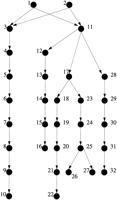
Graph for the partial McKusick pedigree.
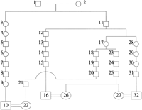
Partial McKusick pedigree (Mkped).
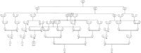
All shortest paths pedigree (ASPped).
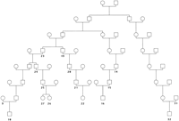
Minimal (Steiner) pedigree.
MKped (Fig. 2) can also be used to illustrate pedigree verification. The paths in MKped that are verified by ASPped (Fig. 3) are as follows: (1) path from 6 to 10; (2) path from 14 to 16; (3) path from 19 to 22; (4) path from 23 to 26 and 27; and (5) path from 29 to 32.
According to ASPped 19 and 23 are siblings, whereas in MKped 18 and 23 are siblings and 19 is a child of 18. This discrepancy is due to an error in MKped—person 18 should not be present in MKped.
The following relationships are verified usingis_child/siblings query features: (1) 5 is the father of 6; (2) 13 is the father of 14; (3) 17 is the mother of 19 and 23; (4) 28 is the mother of 29; and (5) 17 and 28 are siblings.
DISCUSSION
Much attention has been paid toward database management and analysis [e.g., GDB (Fasman et al. 1997), GenBank (Benson et al. 1997), SWISS-PROT (Bairoch and Apweiler 1997)] of genomes as well as to making extensive family trees [e.g., GEDCOM (1997), GED2HTML (1997)] but there is no tool sufficient for a medical geneticist who has a large genealogy as well as genetic information for some of the individuals. Existing software packages [e.g., CYRILLIC (Chapman 1990), DGENE (Lange et al. 1988), Pedigree/Draw (Mamelka at al. 1993), PEDRAW/WPEDRAW (Curtis 1990), PhenoDB (Cheung et al. 1996), SCHESIS (Round 1989)] manage genetic information, store pedigrees, and draw pedigrees but do not automatically extract or verify pedigrees from a genealogy. PEDSYS (Dyke 1992) supports pedigree extraction but not based on the type of optimality criteria implemented in PedHunter. PedHunter provides tools to organize genealogical information in a database and a query facility to access the database. This functionality can create and verify pedigrees according to criteria specified by the user. Advantages of keeping data in a relational database include the following:
-
Simplicity: The concept of a relation provides a self-contained means of representing all types of data relationships using simple tables.
-
Flexibility and Restructuring: There is complete flexibility in database design. Relations can be combined or broken down in other relations with ease.
-
Accessibility and Protection: Keeping data in a relational database provides variable and ready access to all data. Data can be protected and can be used by multiple users.
-
Update: Updating the information in a database is simple because one can verify whether information is consistent. It is important to keep data current for future use.
-
Optimization: A good database design does not duplicate information, which reduces data storage and redundancy.
-
Easy Storage: Physical data storage and logical database structure are independent. There is no worry about where and how the files are stored and they can be accessed using the relational tables.
The usage of PedHunter should be extensible to other existing genealogies besides the Fisher book: (1) There are other genealogy books of the Old Order Amish that overlap with the Fisher book; (2) there are genealogy books of other Amish communities from the midwestern United States; (3) there are genealogy books of other closed North American communities, such as Hutterites and Mennonites; (4) there are genealogies loosely compiled for several island populations and for parts of Finland. Efforts have been initiated to obtain some of these genealogies, to obtain permission to computerize them, and to get the raw data into a computer-readable text file. To usePedHunter on a genealogy, one need only create a database with two tables—person_table andchild_parent_table, as described earlier and use the utility program provided to creategeneration_table.
PedHunter is freely available to scientists studying populations with written genealogies. Interested scientists should send an electronic mail request to richa{at}helix.nih.gov or toschaffer{at}helix.nih.gov. AGDB is intended to be available to scientists conducting National Cancer Institute Internal Review Board (IRB)-approved research on the Old Order Amish. Access to AGDB is carefully controlled and limited by IRB protocol. In the initial phase, the IRB approved usage by five groups that have protocols approved by their IRBs to study the Amish. Each user group is represented by at least one coinvestigator on the protocol for AGDB. More user groups meeting these criteria can be added.
The hunt for disease susceptibility genes has become increasingly automated. One step that has been lacking automated tools is that of connecting distant relatives with the same phenotype into a pedigree for linkage analysis. When the desired pedigree is implicitly part of a large, existing genealogy, computer science techniques can be adapted to extract the pedigree or to verify a putative pedigree systematically. PedHunter provides this automation. The utility of PedHunter is demonstrated by using it to query a database, AGDB, of a large Old Order Amish genealogy. These tools were used to verify and correct parts of a previously published pedigree. The combination of AGDB and PedHunter are immediately useful in ongoing genetic studies of this population (e.g., Stone et al. 1998).
Conversations with geneticists who use the Fisher book suggest that they are content when they can find any pedigree to connect a specified set of individuals. There is no reason to believe that the first pedigree found is the best. In contrast, the all shortest paths and Steiner criteria that PedHunter offers are mathematically rigorous and genetically sensible.
METHODS
AGDB was created in SYBASE SQL Server release 11.0.x of the SYBASE database management software. The functions are implemented using Transact-SQL and C version of Open Client DB-Library.PedHunter was developed on Unix System V release 4.0 running under SunOS 5.5.1 using Sun WorkShop Compiler C 4.2 but it is compatible with other Unix computers. All of the PedHunterfunctions are available as executable files that can be used from the command line prompt; AGDB is available to scientists conducting IRB-approved research on the Old Order Amish. The automatic compilation of the Fisher book genealogy into AGDB was approved by the National Cancer Institute IRB at NIH.
Acknowledgments
This research was performed within the Division of Intramural Research (NHGRI). We thank Dr. Robert Nussbaum for frequent and active encouragement, for helpful guidance about the conventions of genetics research, and for suggestions on this manuscript. We also thank Katie Beiler and our other Amish colleagues and friends in Lancaster County. We are grateful to Gunther Birznieks and Ed Whitley for assistance with SYBASE. We thank Dr. Cyril Chapman, Kevin Crawford, and Dr. Paul Mamelka for their help with CYRILLIC and Pedigree/Draw. We thank Carol Machan for providing the raw data files for AGDB. The research of K.A.H. was supported by a grant (NIH P01HG00373) from the National Center for Human Genome Research.
The publication costs of this article were defrayed in part by payment of page charges. This article must therefore be hereby marked “advertisement” in accordance with 18 USC section 1734 solely to indicate this fact.
Appendix
This Appendix describes the database design, graphs and related terminology, and method used by PedHunter to solve the minimal pedigree, or Steiner pedigree problem.
Database Design
Each person in AGDB is assigned a unique integer, called theprogram id. Utility programs were written to translate from a Fisher id to the program id of the first person in that record, and back from a program id to the Fisher id of one record where that person is listed. There are two central tables in the database—the person table and the relationship table.
The person table (person_table) has information exclusive to the individuals. The columns of this table areprogram id, Name, Birth date, Death date, Address, Gender, Special status, Number of spouses, and Other Information. The Special status field contains information about whether a person is a twin, triplet, foster child, or adopted child. The relationship table (child_parent_table) keeps information relating the individuals. It contains an entry for each couple and a list of their children, if any, in terms of their program idspecified in person_table. The columns of child_parent_table are program id of father, program id of mother, Marriage date, andprogram id of each child. The last field is a list ofprogram ids of each child, if the couple has any. As each row/column combination can have only one value, the list is kept as a string with special delimiters between children.
PedHunter contains a utility program for creating generation_table, which contains the maximum generation level for each person relative to other persons in the database. The two columns of this table are program id of the individual and Maximum generation level. The generation_table is used in computations including inbreeding and kinship coefficients.
Graphs and Related Terminology
A graph is a mathematical representation of objects and the relationship between pairs of objects. Some standard graph terminology is defined below and illustrated by references to the graph in Figure 1. The set of objects represented in a graph are called itsvertices. If two objects are related, they are joined by anedge. For convenience, the following notation is used:
-
V(G) represents the set of vertices for graph G.
-
E(G) represents the set of edges for graph G.
-
e is u–v if edge e joins verticesu and v and the order of u and v is not important. Such an edge is called an undirected edge.
-
e is u → v if edge e joins vertices u and v and the edge is ordered fromu to v. Such an edge is called a directededge.
-
v is in the set V(G) if v is a vertex in graph G.
-
e is in the set E(G) if e is an edge in graph G.
A graph is a directed graph if its edges are directed edges; otherwise, it is an undirected graph. A pedigree can be represented by a graph that has a vertex for each person and an edge for each child–parent pair among the persons in the pedigree. Sometimes it is desirable to make the graph directed by directing each edge from the vertex for parent to the vertex for child. For example, the pedigree (Fig. 2) that is used later as an example, can be represented as in Figure 1. It is useful to view a pedigree as a graph because it traces the passage of genetic information over generations and provides a convenient mathematical representation. A graph representing a pedigree is called a pedigree graph. For the pedigree graph in Figure 1, the set of vertices V(G) is {1,2,. . .,32}, and there are 32 directed edges, including 6 → 7 and 17 → 23.
A path from vertex u to vertex v inG is an alternating sequence of vertices and edges ofG, beginning with u and ending with v, such that no vertex is repeated and every edge joins the vertices immediately preceding it and following it. A path p connectingu to v is denoted p = u, u 1, u 2, …, un, v, where u 1, u 2, …,un is the sequence of other vertices on the path. For example, 1 → 3 → 4 → 5 is a directed path in the graph of Figure 1. The undirected sequence 14—13—12—11—2—3—4—5 is a path in the undirected version of this graph, but not in the directed version. The two paths are denoted as p = 1, 3, 4, 5, and p = 14, 13, 12, 11, 2, 3, 4, 5, respectively.
A directed path p from u to v in a pedigree graph traces one way that v receives genetic material fromu. The vertices on p are also a (partial) list of ancestors of v. Absence of a directed path from u tov indicates that u is not an ancestor of v.Hence, there is no way that v can receive genetic material from u; for example, in Figure 1, person 28 does not receive genetic material directly from person 6, although they have a common ancestor.
A pedigree graph G connects a set of individuals S if there is a vertex in V(G) for each individual in S,and in the undirected version of the graph, there is a path between each pair of vertices representing people in S. The pedigree of Figure 1 is connected. Geneticists usually use the term pedigree to mean a set of parent–child relationships that induce a pedigree graph whose undirected version is connected. Therefore, any formal definition of pedigree constructionshould require that the output pedigree induce a connected pedigree graph. However, this requirement does not specify the output pedigree uniquely, and different specifications of pedigree construction are useful for different purposes.
A cycle is a path that begins and ends at the same vertex. If a graph has no cycles, it is called acyclic. Any directed pedigree graph is acyclic, as the edges are directed from parent to child, and it is biologically impossible to have a cycle in this setting. The term loop is not used here because formally a loop in a pedigree is a cycle in a more complicated, undirected representation called a marriage graph (Lange and Elston 1975). For example, a first-cousin marriage with offspring leads to a loop in the undirected marriage graph but not to a cycle in the directed pedigree graph.
The length of a path is the number of edges in the sequence defining the path; for example the length of pathp = u 0, u 1,u 2, …, un is n. A path from vertex u to vertex v is a shortestpath if it has minimum length of any path from u tov. The length of a shortest path from u to vis also called the distance d(u,v) from u tov.
A shortest path from u to v makes the fewest assumptions about how an allele could have passed from uto v. By the principle of parsimony, a hypothesis that a disease-causing allele passed from u to v requires consideration of all shortest paths from u tov. This observation motivates the asp pedigree construction query.
If G and H are graphs, then H is asubgraph of G if and only if V(H) is a subset of V(G) and E(H) is a subset of E(G).
Given a pedigree graph G that connects a set of peopleS, it is sometimes useful to find a subgraph of Gthat still connects S. One such situation is when the pedigree graph has too many edges to be drawn comprehensibly. A subgraph ofG that contains minimum number of vertices and connectsS is called a minimal subgraph, and the problem of finding a minimal connected subgraph is called a Steiner treeproblem in the computer science literature. Therefore, a minimal pedigree subgraph that connects specified individuals is called aSteiner pedigree. PedHunter finds Steiner pedigrees with the query called minped. Steiner pedigrees are useful for drawing and for linkage analysis when the pedigree graph has too many edges. PedHunter’s method to construct Steiner pedigrees and some background from the computer science literature are explained in the next section.
Steiner Pedigree
Steiner tree problems are widely studied due to applications such as designing road networks and VLSI chips. A survey of Steiner tree problems can be found in Hwang and Richards (1992). Many Steiner tree problems are quite intractable computationally, but pedigree graphs have special features that may make the problem easier. Pedigree graphs are acyclic, and the vertices that must be included typically represent children at the bottom generation. Such vertices that have no outgoing edges are called terminals. In a recent paper Zelikovsky (1997) studied the Steiner tree problem for all directed acyclic graphs with the constraint that the vertices to be connected are terminals. This problem has applications outside genetics. Zelikovsky showed that this version of the Steiner tree problem is intractable in a formal sense and gave an approximation algorithm for the problem. Anapproximation algorithm finds a subgraph that contains all of the prescribed vertices whose size is bounded relative to the size of the minimal subgraph, where the size of a graph is the number of vertices in the graph. However, both the performance ratio and the computation time of this approximation algorithm grow exponentially with the length of the longest path in the graph.
Instead of Zelikovsky’s approximation algorithm, PedHunteruses an algorithm that finds an exact smallest subgraph (subpedigree) as measured by the number of vertices (individuals). The approximation algorithm may be inadequate for the subsequent linkage analysis.
The exact algorithm applies a general technique called branch and bound, which is commonly used to explore exponential-size search spaces in intractable search problems (Papdimitriou and Steiglitz 1982). Branch and bound works well in problems where one can quickly get to a good solution. The weight of the known solution can be used to eliminate many partial solutions whose weight is larger (for a minimization problem such as Steiner tree). When a partial solution is eliminated, all full solutions containing that partial solution are implicitly eliminated also. Branch refers to steps that expand the current partial solution by branching in the search space; bound refers to using a known solution as a bound.
Branch and bound algorithms start by finding an initial solution, keep track of the current best solution, and probe other solutions until it is possible to determine that the current solution is at least as good as any other solution. Branch and bound algorithms typically useretracing or backtracking, which means that part of the current (partial solution) is removed, and the algorithms proceed to consider other solutions that do not contain the removed part. To describe a specific branch and bound algorithm one must describe (1) What makes one solution better than another? (2) How to find an initial solution? (3) How to probe all solutions? For the minimal pedigree problem, the algorithm solves the three basic questions as follows.
Comparing Solutions
The number of edges in the solution is the measure for comparing solutions and the solution with fewer number of edges is better. The number of edges in a solution is called the cost of the solution. The problem statement asks to minimize the number of vertices, but any connected graph with no cycles that has eedges, must have exactly e+1 vertices (Even 1979). Therefore, minimizing number of edges is equivalent to minimizing number of vertices. The algorithm transforms the initial Steiner problem where all edges have weight 1 to a related problem where edges may have larger weight. In the weighted version, the cost of a solution is the sum of weights of edges the solution contains.
Initial Solution
The steps for finding an initial solution are as follows:
- 1.
- Start with the specified set of individuals as the vertices in the solution.
- 2.
- For each vertex v in the solution, except the root, that is not connected to a parent, choose a parent p that is present in the input graph. If the parent chosen is not in the solution, add a vertex for p in the solution. Add the edgep → v to the solution.
- 3.
- Repeat step 2 until there is only one vertex in the solution that is not connected to a parent. That vertex is the root of the pedigree.
Probing All Solutions
Every edge in the input graph G is either in the current solution or it is out. The edges are numbered 1, …,|E(G)| such that edgeu → v is preceded in the order by all edges that are incoming into u. Such an order is possible for pedigree graphs because they are acyclic (Even 1979).
Consider the edges in order e = 1, 2, 3, … . Add edge e to the current solution unless it (1) creates an undirected cycle or (2) creates a (partial) solution with higher cost than the current best. When the current partial solution is a full solution (detectable by testing whether number of edges equals number of vertices minus 1), compare its cost to the current best.
There are four cases that need to be specified further.
- 1.
- If the current partial solution is a full solution and it has lower cost than the previous best, replace the best solution and retrace decisions back to the last edge added in. Omit that edge and proceed to look for better solutions.
- 2.
- If the addition of e creates an undirected cycle, then omite and proceed to add more edges.
- 3.
- If the addition of e creates a partial solution with higher cost than the current best full solution, then as in case 1, retrace back to the last edge added in. Omit that edge and proceed forward.
- 4.
- If the last edge was considered and the solution is not full, then as in case 1, backtrack to the last edge added in, omit it and proceed.
All solutions have been considered when retracing returns all the way past edge 1.
The worst-case computation time of the algorithm is exponential in the number of edges in the input graph. The computation time is lowered substantially by reducing the size of the graph to be considered in the branch and bound algorithm. The graph is reduced by three transformations that are applied repeatedly in any order until none of them can be applied:
- 1.
- Replace paths consisting of k + 1 vertices with one incoming edge and one outgoing edge with a single edge of costk. This is valid because in the original graph, either allk edges must be included or excluded from a solution.
- 2.
- Delete unselected terminals with one incoming edge. This is valid because they cannot serve to connect the selected terminals.
- 3.
- Delete edge u → v if there is another path fromu to v. This is valid because the input graph is an all shortest paths pedigree. Therefore, all paths from u tov have the same cost. The vertices on the multiple-edge path cannot lead to a worse solution than using the single edgeu → v and might lead to a better solution.
The first transformation introduces edges whose weight is >1. The third transformation can apply only after the first transformation has created edges of weight >1 because the cost of all paths from u to v is the same. The cost of a solution in the transformed graph is the sum of costs of all edges in the solution. The transformation is reversed to produce the output Steiner pedigree.
Footnotes
-
↵5 Corresponding author.
-
E-MAIL schaffer{at}helix.nih.gov; FAX (410) 550-7513.
- Received September 22, 1997.
- Accepted February 6, 1998.
- Cold Spring Harbor Laboratory Press


