
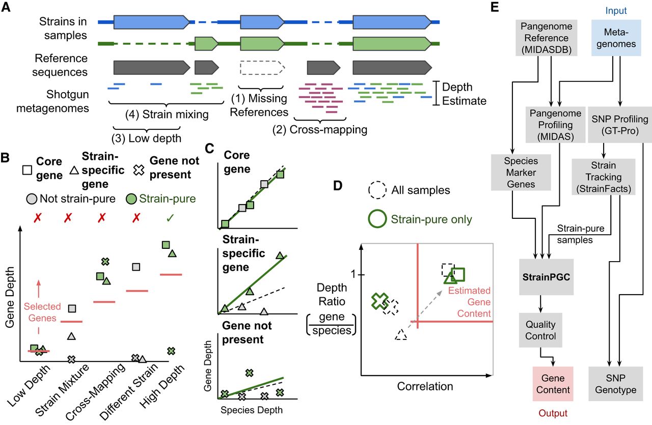
Conceptual overview of strain-resolved gene content reconstruction using StrainPGC. (A) Schematic representation of pangenome profiling, which estimates gene depth based on short-read alignment. The illustration represents profiling of a hypothetical microbial population harboring two strains of the same species (blue and green), each with both shared and strain-specific gene content. Four key challenges for pangenome profiling and gene content estimation are highlighted (brackets; see Introduction). (B) Limitations of gene content estimation using single samples. Depth is shown across five samples for three genes: one gene is ubiquitous across strains (core); another is found in only the strain of interest (strain-specific); and a third is not present in the strain of interest but is susceptible to cross-mapping (not present). Samples are separated along the x-axis and represent five characteristic scenarios: a sample in which the species is not deeply sequenced (low depth), a sample with multiple strains of the species (strain mixture), a sample exhibiting erroneous depth owing to read mapping errors (cross-mapping), a sample with an entirely different strain of the species (different strain), and a high-depth, strain-pure sample (high depth). Colors distinguish between strain-pure samples (green markers) and samples with a different strain or a mixture of more than one strain (gray markers). Traditional, single-sample analysis estimates gene content by selecting genes with a minimum depth (red horizontal line; which is chosen based on the species’ depth). As a result, samples with low depth, cross-mapping, and strain mixing lead to decreased accuracy (indicated with red X's). Only gene content estimation in a strain-pure, high-depth sample without cross-mapping (green checkmark) accurately reflects the strain of interest. (C) Relationship between gene depth and species depth for each of the three genes (panels) across the five samples (marker shape and color as in B). For each, the linear relationship is shown between species depth and gene depth in the set of strain-pure samples (solid green line). We contrast this fit with the linear relationship across all five samples without considering strain variation (dashed line). (D) Schematic depiction of how StrainPGC estimates gene content based on both correlation and depth ratio. The red lines indicate the thresholds of depth ratio and correlation used by StrainPGC to select genes. With all samples combined (dashed markers), the not-present gene is correctly excluded owing to low correlation; the core gene is correctly included, but the strain-specific gene is lost because of its low depth ratio and correlation. Analyzing the strain-pure set separately moves the strain-specific gene into the selection region (dashed arrow), increasing accuracy. (E) Schematic depiction of our integrated workflow to infer gene content across strains using only shotgun metagenomic reads as input.


