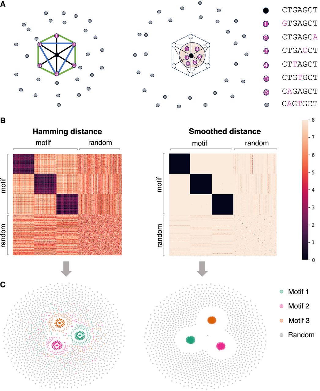
Peculiarities of k-mer manifold. (A) Six motif k-mers (purple dots) with one mutation from the origin (black dot) placed as a hexagon on a circle of radius one, and random
k-mers (gray dots) are placed outside. The Hamming distance between each pair of motif k-mers is two. The Euclidean distance between the dots are two,  , and one for the diagonal (black line), semidiagonal (blue line), and adjacent k-mers (green line). The right panel shows the schematic effects of Hamming distance transformations (Equations 1, 2), in which motif k-mers are pulled closer and random k-mers are repulsed further. (B) Toy example. The left panel shows the Hamming distance matrix of a k-mer (k = 8) data set with three motifs, as highlighted by the black blocks. Within a motif, the Hamming distance ranges from zero
to four. The right panel shows the transformed Hamming distance matrix. After transformation, the distances between the motif k-mers are reduced, whereas the distances between the motif and random k-mers become larger. (C) KMAP visualizations based on the original Hamming distance matrix (left) and the transformed Hamming distance matrix (right).
, and one for the diagonal (black line), semidiagonal (blue line), and adjacent k-mers (green line). The right panel shows the schematic effects of Hamming distance transformations (Equations 1, 2), in which motif k-mers are pulled closer and random k-mers are repulsed further. (B) Toy example. The left panel shows the Hamming distance matrix of a k-mer (k = 8) data set with three motifs, as highlighted by the black blocks. Within a motif, the Hamming distance ranges from zero
to four. The right panel shows the transformed Hamming distance matrix. After transformation, the distances between the motif k-mers are reduced, whereas the distances between the motif and random k-mers become larger. (C) KMAP visualizations based on the original Hamming distance matrix (left) and the transformed Hamming distance matrix (right).