
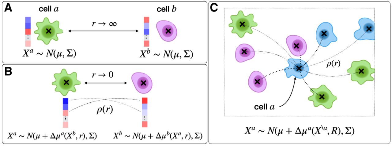
SpaCeNet concept and how it applies to different cellular contexts. (A) A schematic picture of two isolated cells a and b which are infinitely separated (distance r → ∞). In this case, respective cellular profiles with expression levels illustrated in blue and red are modeled by a multivariate
normal distribution with mean expression μ and covariance Σ. The latter encodes the complex coexpression pattern of different RNAs/proteins and facilitates a description
of molecularly diverse cells. (B) A scenario of two neighboring cells, where the cells affect each other; the molecular phenotype changes compared to A as a consequence of the different cellular context. This molecular adaptation of cell a (analogously for cell b) is modeled by a shifted mean expression vector μ + Δμa(Xb, r), where the molecular adaptation depends on the molecular phenotype of cell b and the cell–cell distance r. The molecular adaptation is parameterized by interaction potentials which directly provide estimates of spatial gene–gene
dependencies between gene i and j. (C) A sketch of the more complex scenario of a set of interacting cells. Here, the expression of the cell a is affected by all surrounding cells in a distance-dependent way, as illustrated by thin and bold dotted lines for long-
and short-range interactions, respectively. One should note that the mean expression of the cell a now depends on the molecular phenotype of all other cells  as well as all respective cell–cell distances summarized in R.


