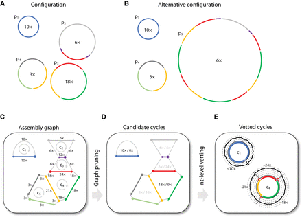
Approach overview. (A) A manufactured example of a latent genome configuration and assembly with eight unique contigs. Contigs are color-coded, and four DNA genomes are marked p1–p4 with their x-coverage specified in their center. For example, p2 has an x-coverage of 6× and contains only three unique contigs, as the short purple contig appears twice. The corresponding assembly graph is shown in C. Under this configuration, cycle c4 is a real cycle that corresponds to p3. (B) An alternative genome configuration that produces the same graph. The presence of the complex genome p5, which corresponds to an involved circuit in the graph, affects the multiplicity of all visited cycles. For example, the multiplicity of cycle c4 is equal to four because the circuit that corresponds to p5 visits the red contig four times while traversing in a loop along the contigs of c4. Note that under this configuration, cycle c4 is a phantom cycle. (C) The assembly graph that corresponds to the configurations shown in A and B. Directed edges appear within a single contig (going from the 5′ end to the 3′ end, represented with arrows) and between adjacent contigs (going from the 3′ end to the 5′ end, represented with dotted lines). The graph contains five cycles (c1–c5), and the x-coverage of edges is indicated. (D) The cycle score σc/τc is specified in the center of each cycle for the graph shown in C. The algorithm recovers all candidate dominant cycles (σc/τc > 1; score colored black) and discards nondominant cycles (score colored gray). For example, cycle c4 has a score of two (σc = 18 × , τc = 9 × ), making it a candidate dominant cycle. (E) In our implementation, nucleotide-level read profiles are computed for all candidate dominant cycles using all paired reads for which at least one side mapped to the cycle, and the algorithm returns dominant cycles with estimates of x-coverage. Reads are grouped into cycle-supporting reads (black line) and nonsupporting reads (red line). For example, the x-coverage of supporting reads along c4 varies, with three short stretches of nonsupporting reads on contig–contig seams. Average read x-coverage values for portions of the cycles are shown on the plot.


