
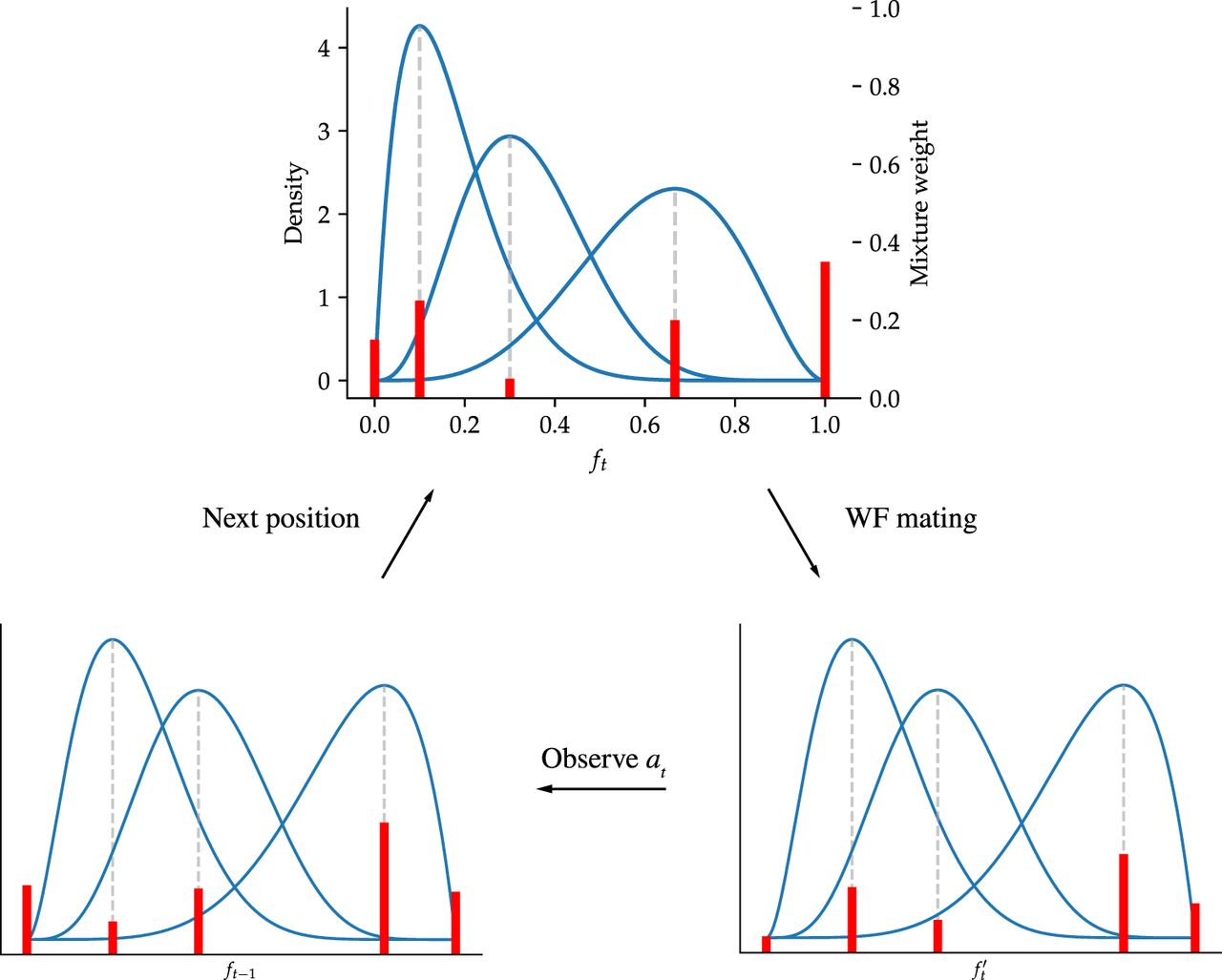
Figure 1.
The bmws model. At each time step t, the latent allele frequency ft is modeled as a mixture of beta distributions, plus spikes at zero and one. In this diagram, there are M = 3 mixture components (blue lines). Mixture weights are indicated as red bars, including the spike weights p0 and p1 at ft = 0 and ft = 1, respectively. After Wright–Fisher (WF) mating, the shape of each beta mixture component, as well as the mixture weights, is updated according to Equation 15. After observing the data at, the mixture weights are again updated according to Bayes’ rule (Equation 16). The process then iterates.


