
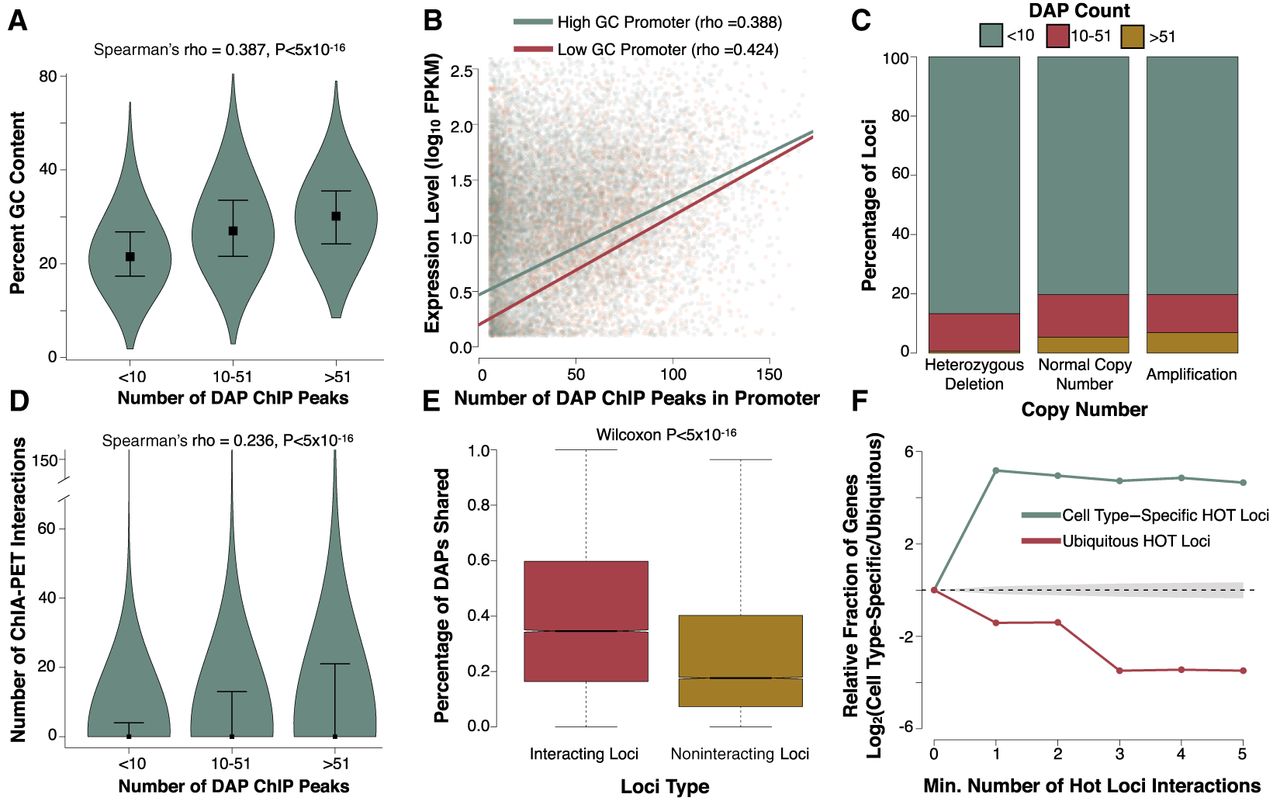
Copy number variation, 3D chromatin structure, and GC content associate with HOT loci. (A) Violin plots showing the GC content of loci with increasing numbers of DAP ChIP-seq peaks. Width of each violin indicates the relative fraction of data contained. Boxes represent the median of each bin and whiskers are drawn to the 25th and 75th percentiles. (B) Scatter plot showing the association between gene expression and DAP ChIP peaks in each genes promoter. Points and trend lines are colored based on promoter GC content. Promoters with GC content in the upper 50th percentile of GC content (high) are colored green, and those in the lower 50th percentile of GC content (low) are colored red. (C) Stacked bar plots showing proportion of loci with various levels of ChIP-derived DAP associations in genomic regions with heterozygous deletions, amplifications, or normal copy number. (D) Violin plots showing the correlation between the number of ChIP-defined DAP associations and the number of Promoter Capture-C interactions. Boxes represent the median of each bin, and whiskers are drawn to the 90th percentile. P-value reported is derived from Spearman's rho correlation of the entire data set. The sample size for each violin from left to right is 194,028, 37,084, and 13,792. (E) Boxplots showing the fraction of DAPs in common between interacting loci and matched noninteracting loci for HepG2 Promoter Capture-C. (F) Line plot indicating the relative fraction (cell type–specific/ubiquitously expressed) of gene promoters with at least the specified number of Promoter Capture-C interactions with other HOT loci. Interactions with cell type–specific loci are shown in green and interactions with loci that are HOT in all three cell lines are shown in red. The gray shaded area represents the 95% confidence, null interval of randomly shuffled loci interactions between cell type–specific and ubiquitously expressed promoters. The 500 cell type–specific and expression-matched ubiquitously expressed genes were identical to those selected in Figure 4.


