
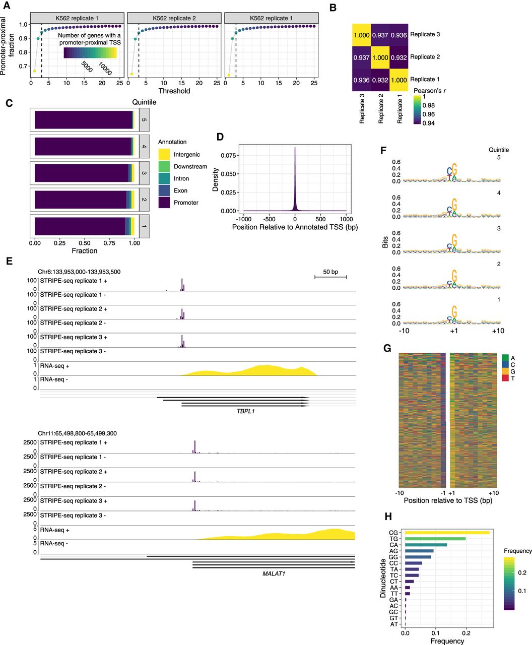
STRIPE-seq profiling of the human initiation landscape. (A) Plot of the fraction of unique TSSs that are promoter-proximal at the indicated read threshold. Dot color and size are indicative of the number of genes with a promoter-proximal TSS. (B) Heatmap of Pearson's r values for pairwise comparisons between TSSs identified in STRIPE-seq samples. Before clustering, samples were thresholded such that each TSS had to have at least 3 raw counts in one sample, and then counts were TMM normalized. (C) Genomic distribution of TSSs in K562 STRIPE-seq replicate 1 broken into quintiles by TSS strength. Genomic distributions of TSSs for all K562 STRIPE-seq samples are presented in Supplemental Figure S19A. (D) Density plot of K562 STRIPE-seq replicate 1 unique TSS positions relative to annotated TSSs. (E) Genome browser tracks showing CPM-normalized STRIPE-seq and poly(A)+ RNA-seq (replicate 1) at two representative regions of the human genome. (F) Sequence logos of TSSs detected in K562 STRIPE-seq replicate 1 broken into quintiles by TSS read count. Sequence logos of TSSs in all K562 STRIPE-seq samples are presented in Supplemental Figure S19B. (G) Nucleotide color plot of the sequence context of TSSs detected in K562 STRIPE-seq replicate 1. TSSs are ranked descending by read count. (H) Dinucleotide frequencies at TSSs detected in K562 STRIPE-seq replicate 1. Dinucleotide frequencies at TSSs in all STRIPE-seq samples are presented in Supplemental Figure S19C.


