
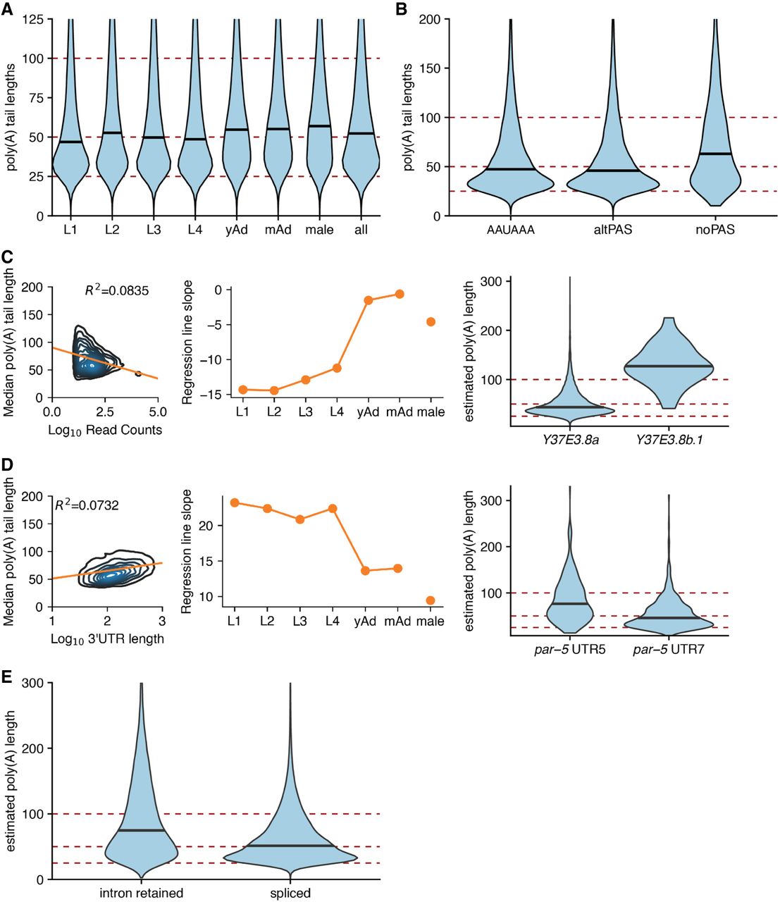
Properties of poly(A) tail length. (A) Violin plot of poly(A) tail length distributions across development. Horizontal black lines show the median of each stage. (B) Poly(A) tail length distributions separated by the PAS type of the associated reads for reads corresponding to isoforms predicted to be coding. (C, left) Density plot showing correlation between poly(A) tail length and expression level by plotting median poly(A) tail length for each isoform versus the log of the expression level of that isoform (across all stages). Linear regression plotted in orange. (Middle) Slope of linear regressions performed on median poly(A) tail length versus expression level data across developmental stages. (Right) Example locus illustrating relationship between poly(A) tail length and expression level Y37E3.8b.1 is less expressed than Y37E3.8a with a longer poly(A) tail length distribution. (D, left, middle) As in the left and middle panels of C, but instead plotting median poly(A) tail length versus the log of the 3′-UTR length. (Right) Example locus illustrating the relationship between 3′-UTR length and poly(A) tail length; par-5 UTR 5 is longer than par-5 UTR 7 and has a longer poly(A) tail length distribution. (E) Violin plots showing poly(A) tail length distributions in fully spliced versus intron retention transcripts.


