
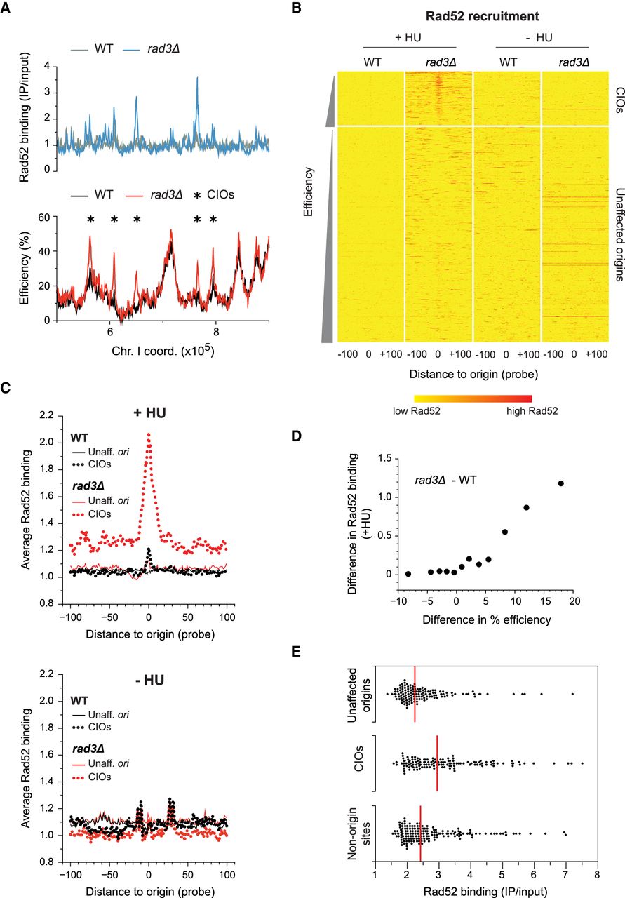
Rad52 is recruited to de-regulated origins. (A) Rad52 binding and origin usage in replication stress conditions. A representative region of the genome is shown. Full Rad52 profiles are in Supplemental Figure S3B; full origin maps are in Supplemental Figure S1C. Top: Rad52 recruitment in wild type (WT, gray) and rad3Δ (blue). y-axis: Rad52 binding (IP/input). Bottom: origin efficiencies for wild type (black) and rad3Δ (red). Asterisks mark CIOs. y-axis: origin efficiency. x-axis for top and bottom: chromosome coordinates. (B) Heat maps of Rad52 binding at origins in HU-treated cells (left) or during an unperturbed S phase (right). Data are from ChIP-chip experiments as in A and Supplemental Figure S3G. Data analysis and presentation are as in Figure 2C. Note that there are a few red horizontal lines in rad3Δ in –HU; these represent high levels of Rad52 recruitment to the end of the right arm of Chromosome III (Supplemental Fig. S3B), which we have not further investigated in this study. (C) Average signal plots of Rad52 binding at origins in HU-treated cells (top) or during an unperturbed S phase (bottom). Data analysis and presentation are as in Figure 2D. Black: wild-type; red: rad3Δ. Solid lines: unaffected origins; dotted lines: CIOs. (D) Correlation between the differences in Rad52 binding and in origin usage between rad3Δ and wild type. Data analysis and presentation are as in Figure 2E. x-axis: difference in origin efficiency; y-axis: difference in Rad52 binding. The nonaveraged data are shown in Supplemental Figure S3E. (E) Levels of Rad52 binding at peaks associated with unaffected origins, CIOs, and nonorigin sites. Each point represents a single origin. Red lines: median values for each category of Rad52 peaks. x-axis: level of Rad52 binding (IP/input).


