
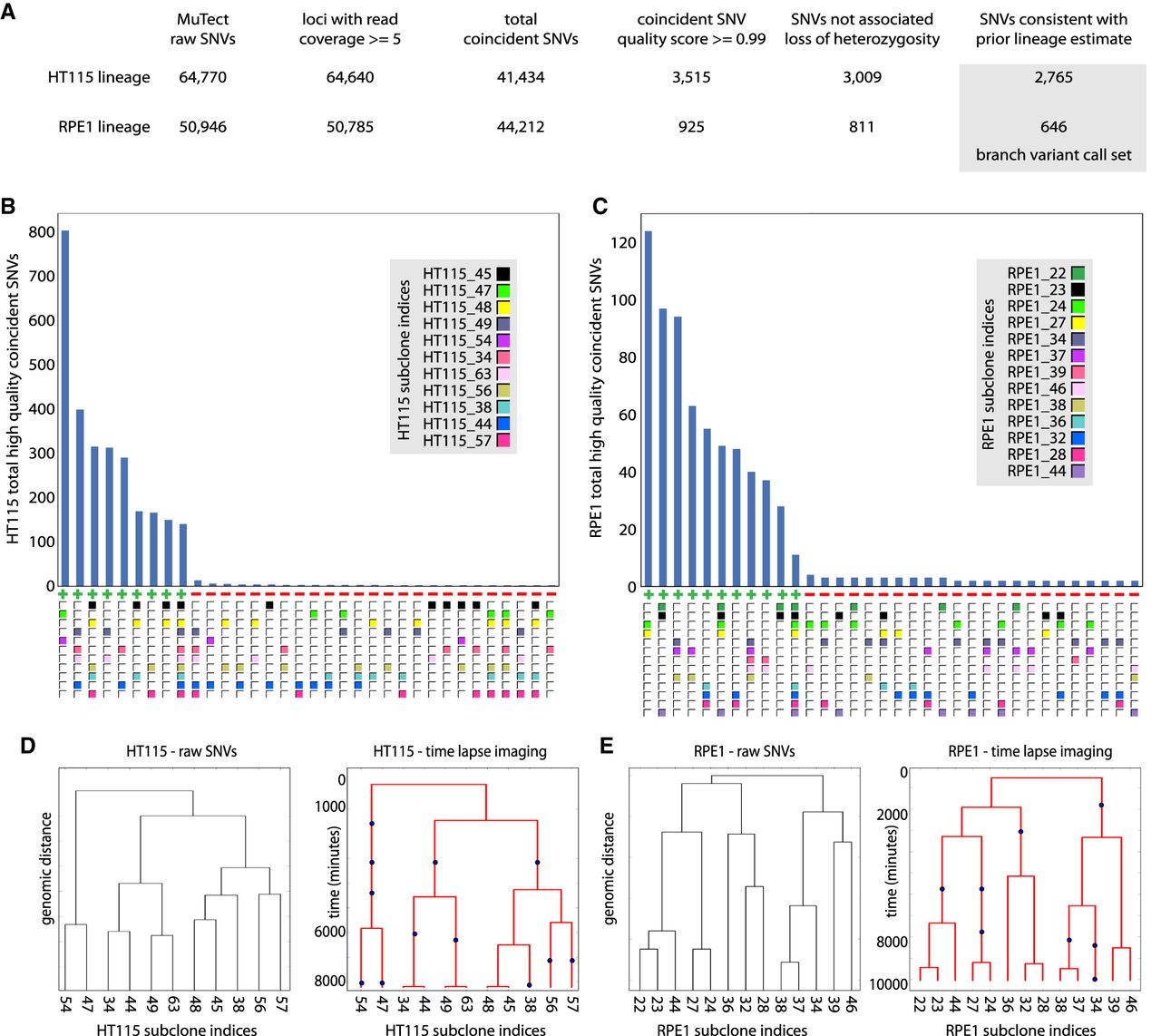
Accuracy and sensitivity of lineage sequencing without microscopic tracking. (A) Scheme of the analysis pipeline for identifying branch variants by the “raw variants → lineage → called variants” approach. Variant counts at different stages of the informatics filtering steps used to identify high-quality lineage structure concordant branch variants are shown for the HT115 and RPE1 lineage sequencing experiments. The pipeline is similar to the “optical tracking → lineage → variants pipeline” (Fig. 2A) except that lineage information is incorporated later, separately from SNV coincidence, and the source of the prior lineage estimate is analysis of raw SNVs (see B and C) rather than time-lapse imaging. (B,C) Histogram of the number of high-quality coincident SNVs for each set of subclones in which such variants occurred for the HT115 (B) and the RPE1 (C) data sets. At bottom, each cluster is marked as consistent (+) or inconsistent (−), with the lineage structure indicated by the time-lapse imaging. For each cell line, the group of subclone sets with high frequencies of these SNVs are both internally self-consistent and consistent with the independent time-lapse imaging data. (D,E) Comparison between dendrograms representing lineages based on genomic distance among subclone pairs and the time-lapse imaging data (only subclones that were cultured and sequenced are represented); HT115 (D) and RPE1 (E). The dendrograms based on genomic distance and time-lapse imaging indicate the same connectivity between subclones, the information relevant to joint variant calling in lineage sequencing, but have different branch lengths and are missing several internal cell divisions. The blue dots in the time-lapse imaging dendrogram represent cell division events that are not independently available from the sequence data. The dendrograms based on time-lapse imaging have a y-axis with units of minutes.


