
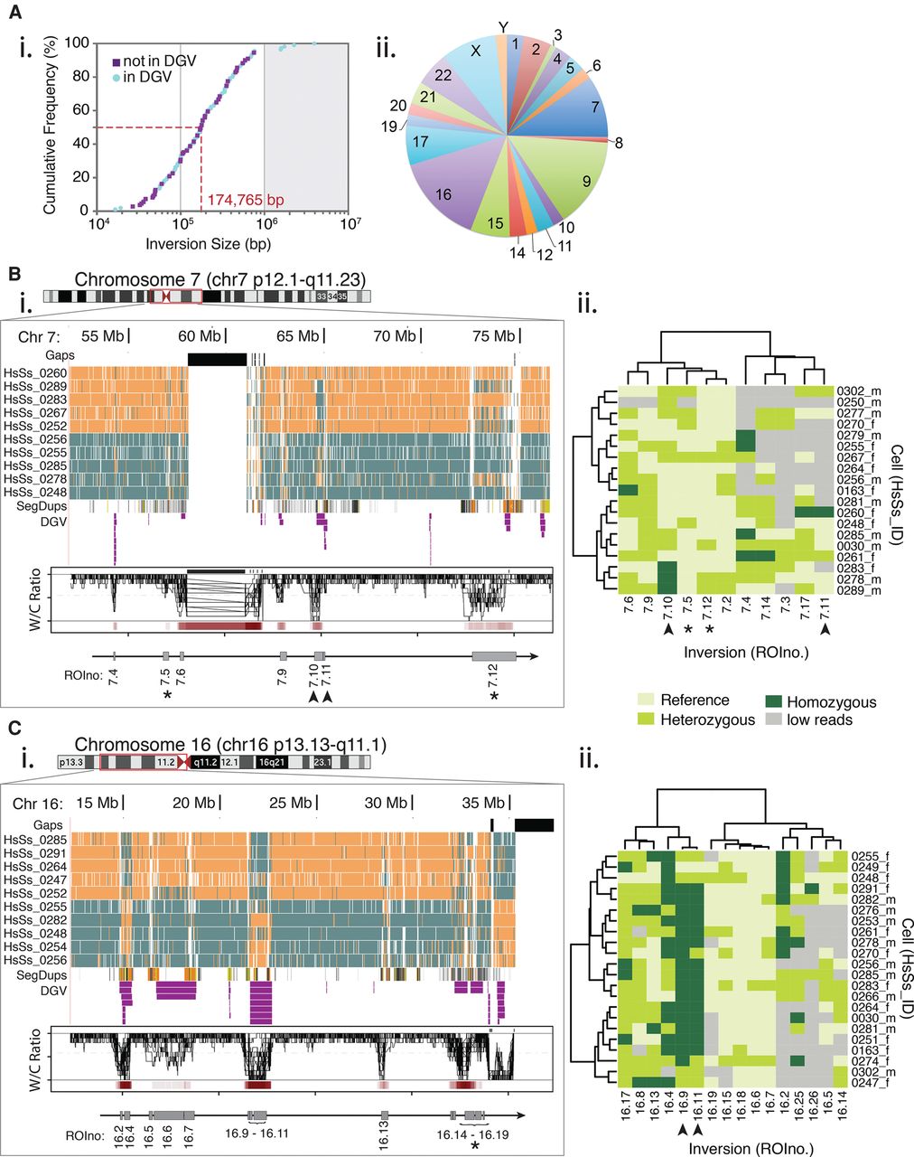
Polymorphic inversions mapped in multiple single cells of a pooled donor population. (A) Size and genomic distributions of 111 polymorphic inversions identified in the pooled donor population. (i) The cumulative frequency of inversion sizes in base pairs (bp), divided into new inversions (purple squares) and those overlapping with the Database of Genomic Variants entries (blue circles). The median inversion size (dashed red line) is well below the 1-Mb detection limit of traditional cytogenetic techniques (gray shading). (ii) Distribution of the total number of inversions present on each chromosome. (B,C) Polymorphic domains (red box) mapped to Chr 7 (B) and Chr 16 (C). Asterisks and arrowheads denote specific inversions highlighted in the main text. (i) Detail of the domains shown in the UCSC Genome browser ‘packed’ view for 10 representative Strand-seq libraries, along with tracks for sequence gaps (black), segmental duplications (SegDups), and inversions identified in the DGV (purple). Corresponding overlaid Invert.R histograms of W/C ratios and inversion frequency heat maps (red bars) are shown in the lower panel. The polymorphic inversions (gray boxes) and corresponding ROIno identifiers are shown below. (ii) Clustered heat maps of the genotyped inversions (x-axis) identified in each cell (y-axis). Inversions are depicted as pale green (homozygous reference), medium green (heterozygous), or dark green (homozygous). In some cases, too few reads were present in the region to genotype the ROI (gray).


