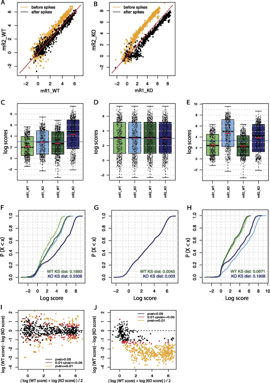
Spike adjustment improves similarity between replicates and reveals genuine differences in Pol III occupation. (A,B) Scatter plots showing the relation of Pol III loci scores between the two WT (A) and the two Maf1 KO (B) replicate samples before (orange) and after (black) spike adjustment. The red line corresponds to x = y. (C–E) Boxplot representations of the Pol III loci score distributions for the two WT samples (light and dark green, mR1_WT and mR2_WT) and the two Maf1 KO samples (light and dark blue, mR1_KO and mR2_KO). The scores were normalized to total number of tags aligned onto the genome (C) followed by either quantile normalization (D) or spike adjustment (E). (F–H) Empirical cumulative frequency distributions functions (ECDFs) of the log scores of the indicated distribution. Samples were normalized to the total number of tags aligned onto the genome (F) followed by either quantile normalization (G) or spike adjustment (H). The Kolmogorov-Smirnov (KS) distance for the two WT (green lines) and the two Maf1 KO (blue lines) samples is shown at the bottom right of each panel. (I,J) Mean difference scatter plots illustrating Pol III occupancy in WT and Maf1 KO livers. Samples were normalized to the total number of tags aligned onto the genome followed by quantile normalization (I), respectively by spike adjustment (J). Scores for WT and KO conditions are the average of the two replicates. Loci with scores showing a significant difference in the WT versus Maf1 KO samples are represented with yellow (P ≤ 0.01) and red (0.01 < P ≤ 0.05) dots.