
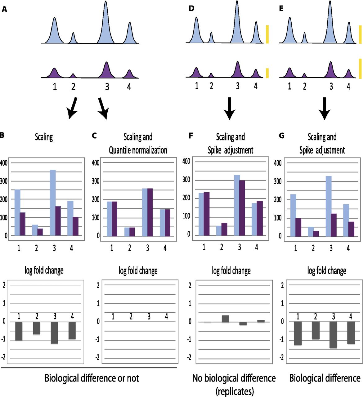
Normalization can obscure global effects. (A) Schematic representation of peaks obtained after ChIP-seq in a hypothetical example where all peaks are uniformly diminished in the second (purple) sample compared with the first (light blue). These samples can represent a replicate experiment, in which case the overall decrease observed in the second sample is the result of experimental variation, or they can represent experiments performed with samples collected under different conditions, in which case the global decrease might reflect a biological difference. No spike chromatin is included. (B) Normalization by scaling to total number of tags aligned onto the genome (i.e., normalization for sequencing depth) showing tag counts (top) and log2 fold change (bottom). In this hypothetical example, the number of tags aligned onto the genome is quite similar in both samples, and this type of normalization indicates a general decrease for each peak in the second sample, whether the two samples are biologically different (and thus should indeed indicate a protein occupancy decrease in sample 2) or similar (and thus should in fact display similar signals). (C) Normalization by scaling followed by quantile normalization showing tag counts (top) and log2 fold change (bottom). In this example, the second step—quantile normalization—will equalize the sample distributions whether the samples are biologically different or not, because the decrease in sample 2 is uniform. In D and E, spike chromatin is included in the sample and gives rise to signals symbolized by the yellow bars. (F,G) Normalization by scaling followed by spike adjustment showing tag counts (top) and log2 fold change (bottom). In F, the spike adjustment factor increased the signals in sample 2 by a factor of about two, in G, the spike adjustment factor decreased the signal in sample 2 by a factor of about 0.8 (see yellow bars). Spike adjustment reveals whether the samples are in fact similar (example in F) or are in fact biologically different (example in G).


