
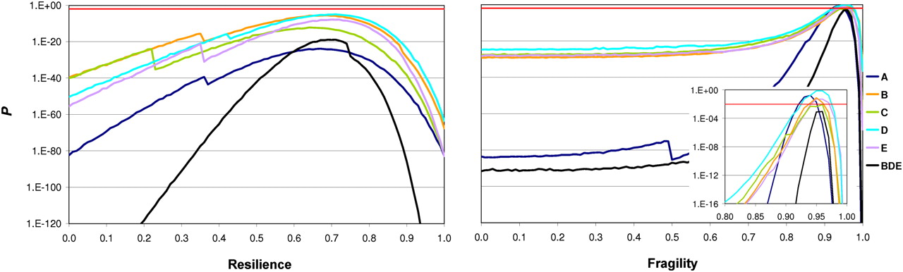
Assessment of the feasibility of two extreme modes of chromosome evolution to explain the observed patterns of change for different Muller's elements (A–E). The particular ways in which resilience and fragility were simulated correspond to R2 and F1 (Supplemental Table S30). (Left) P-values from the G-tests goodness-of-fit performed to evaluate the deviation of the observed distribution of the number of different neighboring orthologous landmarks and that resulting from simulations under different degrees of resilience (r ∈ [0, 1]). The observed and the simulated distributions show a poor fit even for that degree of resilience (r = 0.68 ± 0.03) for which the best fit between them (i.e., the largest P-value) is obtained. (Right) P-values from the G-test goodness-of-fit performed to evaluate the deviation of the observed distribution for the size of orthologous landmarks and that resulting from simulations under different degrees of fragility (f ∈ [0, 1]). If f = 0, the simulated evolutionary scenario is equivalent to the random breakage model. If f = 1, only the IGA edges flanking the 2683 + 5 inter-IGA regions chosen at random are flagged as fragile and can appear at the limit of chromosomal rearrangements. The observed and the simulated distributions do not show statistically significant differences for Muller's elements A, B, D, and E when f = 0.95 ± 0.01. For Muller's element C, there is a marginally significant difference, and for the combined Muller's element (B + D + E), P < 9 × 10⁻⁴. The statistical significance level is set to 0.01 (red horizontal line) because of the necessary correction for multiple testing. For each Muller's element and resilience/fragility value, 1000 simulations were done in which IGA order was reshuffled by a number of inversions equal to that estimated with MGR. Both the parameters of resilience and fragility were sampled with steps of 0.01. The William's correction was applied to all the G-tests performed.


