
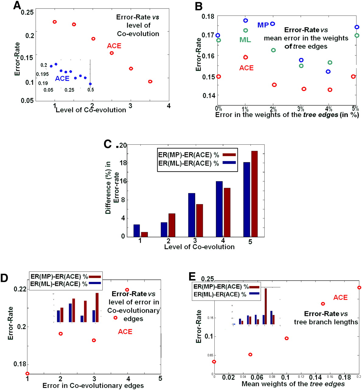
Summary of the simulation results, reporting the mean over 10 runs using coevolutionary forests with 100 trees, each with 20 leaves and branch lengths in the range of from 0.1 to 0.4. (A) The error rate (frequency of sites inferred with error, y-axis) vs. the level of coevolution (normalized by the number of trees, x-axis). The inset shows the typical behavior at very low levels of coevolution. (B) The error rate vs. errors in the weights of the tree edges. (C) Difference between the error rate of ACE and the error rate of MP or ML (in %) vs. level of coevolution. (D) The error rate vs. error in the coevolutionary graph, the latter denoting the mean number of coevolutionary edges changed between a node (representing an organism) and its descendant in the evolutionary trees; the ACE was based on the coevolutionary graph in one of the nodes. The inset shows the difference (in %) between the error rates vs. the error in coevolutionary edges. Note that the gap between ML and ACE decreases when the error in coevolutionary edges increases. (E) The error rate vs. mean weight of the tree edges. The inset shows the difference (in %). Note that the gap between ML/MP and ACE increases when the mean weight of the tree edges (the probability to gain/loss a protein) increases.


