
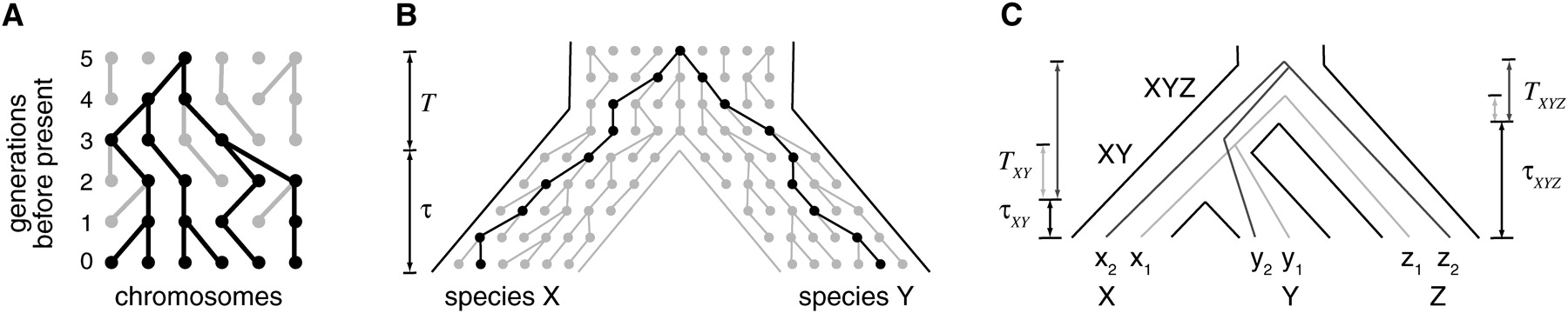
(A) Illustration of a genealogy under the simple Wright–Fisher model. Each row of circles represents the set of individual (nonrecombining) chromosomes in a constant-sized population during a discrete generation. Edges between circles represent inheritance relationships. Under this model, each individual chromosome randomly samples a parent from the previous generation. As a result, the present-day individuals are related by a tree, known as a genealogy, consisting of those individuals and all of their ancestors (black). Notice that many ancestral chromosomes have no present-day descendants. (B) Population genetic interpretation of speciation, assuming discrete generations. At a time τ generations before the present, the population was abruptly partitioned, and the precursors of species X and Y became genetically isolated. Individuals from the two species are related by a genealogy that reflects both this speciation event and the genealogy of their ancestors in the population at the time of speciation. Their time to most recent common ancestor (t) can be decomposed into a time since speciation (τ) and a time since coalescence (T). (C) A three-species phylogeny for species X, Y, and Z, with ancestral species XY and XYZ. Individuals x1, y1, and z1 have a genealogy that reflects the species tree (light gray), but individuals x2, y2, and z2 have a genealogy with a discordant topology (dark gray).


