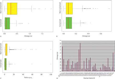
(A–C) Box plots representing the distribution of the ω values (A,B) and the ratio ωf/ωs (C). The first quartile right boundary is the left border of the box, the red line is the median, and the third quartile right boundary is the right border of the box. (A) The distribution of the flanks ω values, nonconserved, first quartile boundary: 0.105, median: 0.251, third quartile boundary: 0.505. Conserved, first quartile boundary: 0.015, median: 0.071, third quartile boundary: 0.211. There is a significant difference between the conserved and nonconserved groups (P = 3.275 × 10⁻¹², two-sample Kolmogorov–Smirnov test). The nonconserved data set contains three ω values of 1.0 × 10⁶; these values were removed from the plot to allow improved inspection/comparison of the two distributions. (B) The distribution of the shadow’s ω values, nonconserved, first quartile boundary: 0.04, median: 0.078, third quartile boundary: 0.145. Conserved, first quartile boundary: 0.039, median: 0.075, third quartile boundary: 0.132. There is no significant difference between the conserved and nonconserved groups (P = 0.961, two-sample Kolmogorov–Smirnov test). (C) Nonconserved, first quartile boundary: 2.203, median: 3.254, third quartile boundary: 5.752. Conserved, first quartile boundary: 0.122, median: 2.115, third quartile boundary: 4.119. There is a significant difference between the conserved and nonconserved groups (P = 9.115 × 10⁻¹¹, two-sample Kolmogorov–Smirnov test). (D) The ω values for the conserved and nonconserved flanking regions in the protein alignments that contained both conserved and nonconserved repeats. There is a significant difference between the conserved and nonconserved groups, and the nonconserved flanking regions are under less purifying selection compared with conserved flanking regions (P = 3.7 × 10−183). Of note are the four proteins whose nonconserved flanking regions may be undergoing adaptive selection (ω > 1).


