Spectral Biclustering of Microarray Data: Coclustering Genes and Conditions

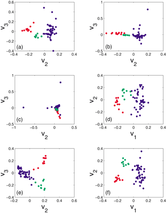
Lymphoma: Scatter plot of experimental conditions of the two best class partitioning eigenvectors v_i,v_j. The subscripts (i,j) of these eigenvectors indicate their corresponding singular values. CLL samples are denoted by red dots, DLCL by blue dots, and FL by green dots. (a) Bistochastization: the 2nd and 3rd eigenvectors of BB^T . (b) Biclustering: the 2nd and 3rd eigenvectors ofR ⁻¹ AC ⁻¹ A^T . (c) SVD: the 2nd and 3rd eigenvectors ofAA^T . (d) Normalization and SVD: the 1st and 2nd eigenvectors of ĀĀ ^Twhere Ā is obtained by first dividing each column of A by its mean and then standardizing each row of the column normalized matrix. (e) Normalized cut algorithm: 2nd and 3rd eigenvectors of the row-stochastic matrix P. P is obtained by first creating a distance matrix S using Euclidean distance between the standardized columns of A, transforming it to an affinity matrix with zero diagonal elements and off diagonal elements defined asW_ij  = exp(−αS_ij )/max(S_ij ) and finally normalizing each row sum of the affinity matrix to one. (f) As in (c) but with an SVD analysis of the log interaction matrix K instead of A.