
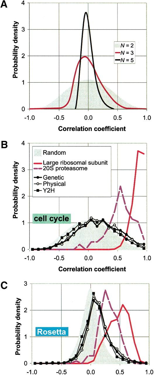
Distributions of correlation coefficients between expression profiles. In A, we show distributions of the average correlationρ̄N of N genes for the cell cycle experiments. The gray curve in the background represents the caseN = 2 (i.e., simply the distribution of pair-wise correlations). In the case of N >2,ρ̄N is defined as the average of all possible (N 2−N)/2 pairwise correlations among theN genes. We show here, as examples, the distributions forN = 3 and N = 5. The distributions obviously become narrower, reflecting the fact that it becomes more unlikely to find large groups of strongly correlated genes at random as Nincreases.
These distributions provide a suitable control for the observed correlations between pairs of genes (N = 2) or for the average correlations among the subunits of a complex (N>2).
We have developed a method to efficiently sample the distribution curves f(ρN) (see Methods). Based on the distribution function off(ρN) we can calculate a one-sidedP-value:
 This P-value then represents the chance that a group of N randomly selected genes could exhibit an average correlation greater than or equal to that of a complex with Nproteins (see Fig. 3).
(B and C) The distribution of pair-wise correlations for both the cell cycle (Cho et al. 1998) and the Rosetta experiments (Hughes et al. 2000) in two protein complexes (the ribosome and the proteasome) as well as for the aggregated data sets (genetic, physical and yeast two-hybrid). The gray curves in the background are the control distributions for N = 2 as explained above. The distributions for the ribosome and the proteasome are strongly shifted to the right of the control; this effect is much weaker for the data sets of aggregated interactions.


