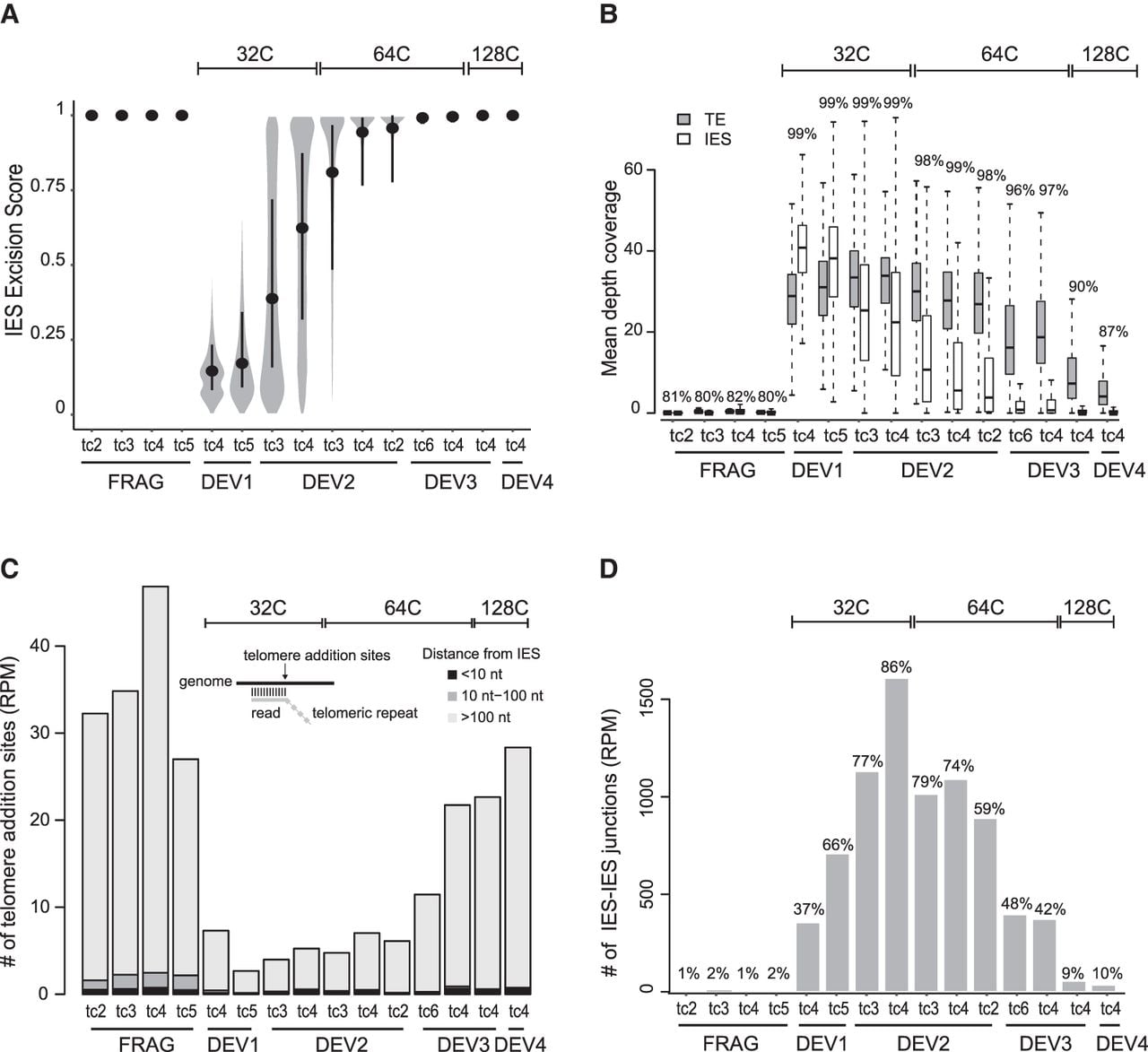
Kinetics of precise IES excision and imprecise DNA elimination. (A) Distribution of ESs in all samples. Samples are named and ordered according to developmental stage (DEV1 to DEV4), time course (tc2, tc3, tc4, tc5, tc6), and C-level (indicated above the plot). Hierarchical clustering of ESs confirmed that samples from the same developmental stage (DEV1 to DEV4) group together (Supplemental Fig. S4C). Inside each developmental stage, for a given C-level, we have ordered the samples using their median ES score. For each time course, old MAC fragments (FRAG) were also sorted as controls. The black dot is the median, and the vertical black line spans the second and third quartiles. (B) TE and IES coverage during autogamy. The mean depth coverage distribution is represented as a boxplot. For each data set described in A, the gray boxplot shows TE coverage; the white, IES coverage. The percentage of the MIC genome covered by the sequencing reads is indicated above each pair of boxplots. (C) Abundance of telomere addition sites during autogamy. The schema above the bars illustrates the method for detection of telomere addition sites using the sequencing data. For each data set, the bar shows the normalized number (per million mapped reads [RPM]) of detected telomere addition sites localized at <10 nt (black), between 10 and 100 nt (dark gray), and >100 nt (light gray) from an IES. (D) Quantification of IES–IES junctions. All putative molecules resulting from ligation of excised IES ends (see Supplemental Fig. S5A,B) are counted and normalized using sequencing depth. The percentage of IESs involved in at least one IES–IES junction is indicated above the barplot.